Tutorials

Every TimeCues workflow has a complete step-by-step written walkthrough on this page — each one illustrated with screenshots of the actual UI, and ready to follow today. Click any card below to jump straight to its tutorial, or use the page outline on the right. Video screencasts will land over time.

There is also a full reference for every flag, environment variable, and Docker compose profile at the bottom of this page — the “what do I actually type and which knobs exist” companion to the workflow guides.

If there’s a screencast you’d like recorded first, say so on the contact page.

Getting started in 3 minutes

Open a song, scrub the waveform, drop your first boundary, save. The shortest possible loop through the app.

Read the walkthrough →

Creating a new dataset

From a fresh deploy to your first reviewed corpus — claiming the workspace, uploading audio, picking an access tier, inviting your team, and switching between datasets.

Read the walkthrough →

Aligning the beat grid

Bar-start anchor, Grid Offset, Steady vs Mapped vs Hand-placed modes, what to do with songs that drift, and how to read the red / amber / emerald grid-readiness glyph.

Read the walkthrough →

Mapped & hand-placed tempo

For songs whose count restarts partway through, and for the beats that refuse to line up — build a tempo map, or pin individual beats by hand on top of a base grid.

Read the walkthrough →

Annotating boundaries with the keyboard

The full keyboard-driven flow — M to add, snap-to-grid, the violet-halo tick when you snap, undo/redo, and how to think about the layer cards in the sidebar.

Read the walkthrough →

Comparing algorithms

Toggle algorithm overlays, read the per-song F-measure and HitRate, and switch reference layers to see how scores shift.

Read the walkthrough →

The Auto-guess workflow

Generate an AutoGuess from the four clustered algorithms, then tick through point-by-point with ✓ / ✗ / @ to harvest a clean manual layer in a fraction of the time.

Read the walkthrough →

Writing a custom detector

Drop a Python file in tools/python/custom/, reload, and have your algorithm show up as an overlay with full evaluation. No build step.

Read the walkthrough →

Multi-annotator: comparing two people's work

Signing in, the per-annotator namespace, side-by-side comparison view, and resolving disagreements between annotators.

Read the walkthrough →

BPM auto-detection chips

The five detectors (librosa + CPJKU-madmom), what the clickable chips do, and how to pick the right candidate when they disagree.

Read the walkthrough →

Stem separation with Demucs

Triggering the stems daemon, what the wait time looks like, and using the resulting vocal / drum / bass / other tracks in inspection.

Read the walkthrough →

Self-hosting on your own server

Bring up the Docker stack on any VM or homelab, put a TLS reverse proxy in front, and claim the first admin.

Read the walkthrough →

Settings — the complete tour

Every panel, every toggle, every dropdown — the role banner, the five categories (User info / Annotation / Research / Corpus management / Danger Zone), what's admin-only, and where to flip each one.

Read the walkthrough →

Want one sooner?

The order above is roughly priority-first. If there’s a specific workflow you’d find most useful — or a wrinkle in the app that confused you and would benefit from being shown rather than written — drop a note on the contact page and I’ll bump it up.

---

Step-by-step tutorials

The detailed walkthrough for every card above, plus a flags / settings / compose-profile reference at the end. Skim the one that matches what you want to do — each section is self-contained and references the deep-dive part of the user guide when the topic deserves more than a screencast can give.

⚠ Set BPM and lock the grid in Dataprep before anything else. Every annotation snaps to the song’s beat grid, and the Annotator Tool refuses to open without a BPM. The grid-readiness glyph on the song row in the sidebar turns emerald ♩ once you’re ready; amber ♩ means the grid is not locked yet, red ♩ means BPM is still missing.

Getting started in 3 minutes

▶ Getting started — a tour of TimeCues Studio

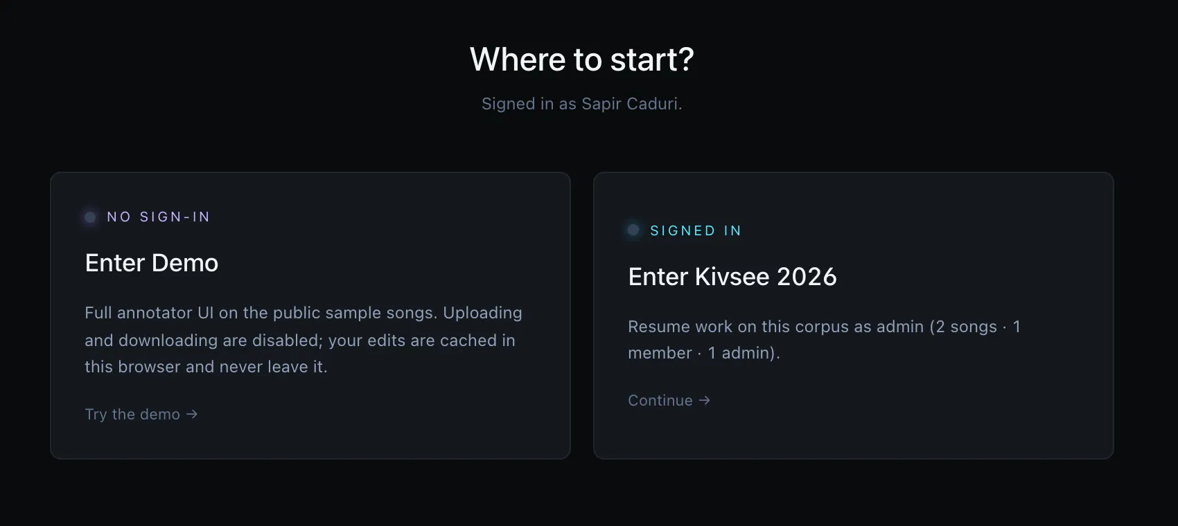The main page — “Enter Demo” to look around with no account, or “Start a new dataset” / “Enter your corpus” to work on real audio.

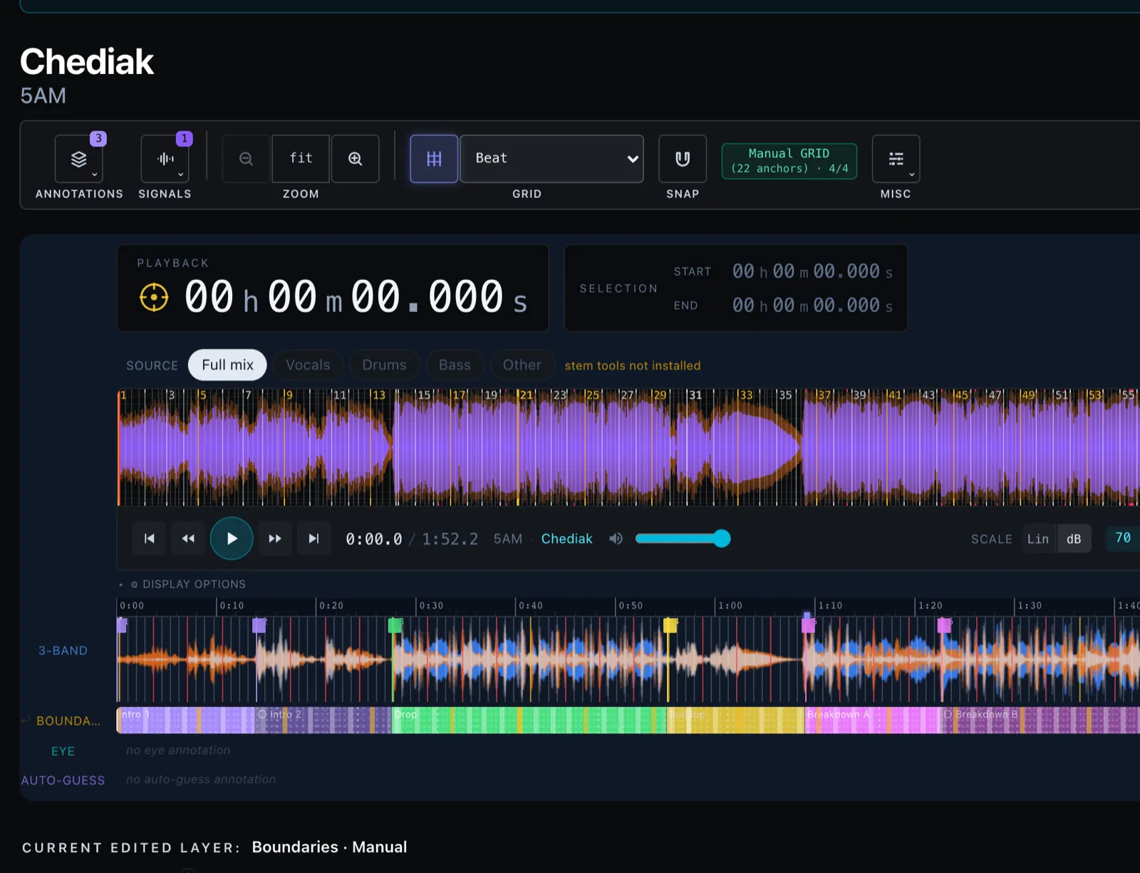The Annotator Tool — press space to play and M at each transition to drop a boundary on the nearest beat.

The shortest possible loop through the app — open a song, lock the grid, drop your first boundary, save.

1. Open the app — the live demo if you just want to look, or your own deploy from docker compose up. The main page shows two entry cards: Enter Demo and either Start a new dataset (fresh deploy) or Enter <corpus> (already claimed).
2. Sign in or click Enter Demo. Demo Mode needs no account and keeps every edit in localStorage; signing in writes annotations server-side under your annotator id.
3. You land in Dataprep. Pick a song in the left sidebar. If the manifest is empty, drop an MP3 into the upload zone.
4. Open step ① Tempo in the Song setup sidebar on the right. Click an Auto-detected chip (or type a value) to set BPM. Then in step ② Downbeat, press G (or click Set bar 1 here) at the first audible kick to align bar 1.
5. Switch to the Annotator Tool tab. The song’s sidebar glyph should now read emerald ♩.
6. Press space to play, press M when the song hits a section transition. The boundary lands on the nearest beat; tab to give it a label.
7. Auto-saves on every edit. No save button. Refresh — the boundary is still there.

What you need: Nothing beyond docker compose up — or just open the live demo, which needs no account and no install. No profile and no flags: this is the core loop, on by default.

Creating a new dataset

▶ Prepare a dataset — tempo, grid, and the team

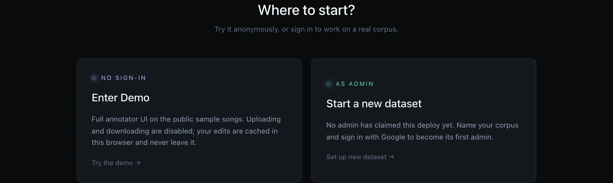On a fresh deploy with no corpus yet, the second card reads “Start a new dataset” — claiming the corpus on disk and making your account its first admin.

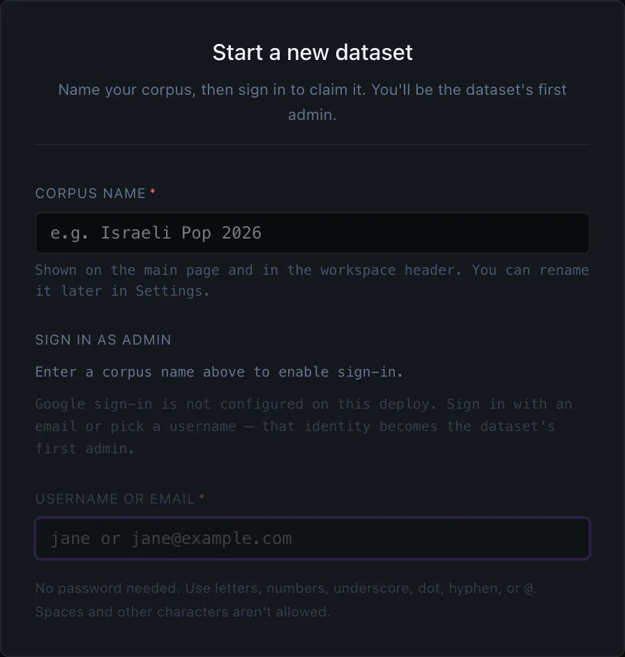The setup form — name the corpus, then sign in (Google, or an email / username when Google isn’t configured) to claim it as the first admin.

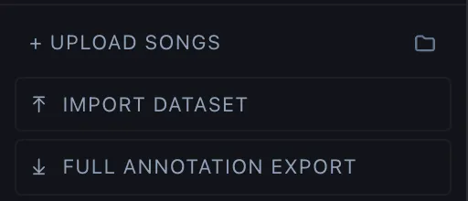Upload songs, import an existing dataset, or export — all from the sidebar header.

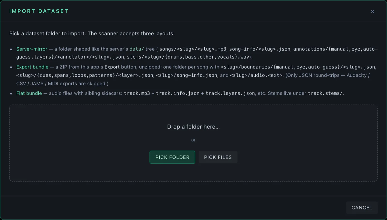The Import dataset dialog — bring an existing folder of songs into the corpus.

From a fresh deploy to your first reviewed corpus. This is the “day-zero” path — the first thing you do on a TimeCues install where nobody’s claimed the workspace yet.

Demo vs. claimed corpus

The landing page after sign-in shows two cards, so know which one you want:

• Enter Demo — uses the three CC0 songs shipped in data-default/songs/ (edm-at-midnight, pantheon, phonk-remix) with pre-computed BPM, grids, stems, and one Manual layer per song. Every edit lives only in your browser’s localStorage — nothing hits disk. Use this to evaluate the tool with zero commitment; reset by clearing site data.
• Start a new dataset (fresh deploy) — claims the corpus on disk for your annotator id, with you as the first admin. Audio uploads, annotations, and BPM caches all persist to data/songs/, data/annotations/, and data/algorithm-outputs/.
• Enter <corpus name> (already-claimed deploy) — the corpus exists; you’re joining as whatever tier the admin set for your email. If your email isn’t on the allowlist you’ll see a Public-tier read-only view of the demo songs only.

Step by step — creating from scratch

1. Open the app at your deploy URL or the live demo. If this is a fresh deploy the landing page will show Start a new dataset. If someone’s already claimed it you’ll see Enter <corpus> and need that admin to add you to the team.
2. Click Start a new dataset. You’ll be prompted to sign in via Google. Your email becomes the first admin’s id; in dataset-config.json it lands under peopleByEmail[<you>].tier = "admin".
3. Name the corpus. This is the human-readable string that shows in the sidebar title and the Enter <corpus> card. Stored at data/dataset-config.json:datasetName. Edit later from Settings → Corpus management → Admin & access.
4. You land in Dataprep with an empty song list. The viz canvas shows a placeholder.
5. Drop audio into the upload zone at the bottom of the song sidebar. MP3, WAV, FLAC, and M4A are supported; the file’s slug is derived from the filename (lowercased, non-alphanumeric → -), and the file lands at data/songs/<slug>/<filename>.<ext>. Drag-drop multiple files at once to bulk-add — each one becomes its own song row.
6. Click a song in the sidebar to open it. The waveform draws, the audio decodes. If you uploaded files with embedded ID3 metadata the Song Info Bar pre-fills title and artist.
7. Lock the grid for this song. Work through the Song setup sidebar’s numbered steps (see Aligning the beat grid below). The sidebar’s per-song workflow glyph flips from red ♩ to amber ♩ once BPM is set, and to emerald ♩ once you’ve confirmed the grid by anchoring the bar start.
8. (Optional) Invite the team. Go to Settings → Corpus management → Admin & access → People and add emails one row at a time. Each row chooses one of four tiers — admin, researcher, team, public. The added person sees the dataset the next time they sign in. See Roles in the user guide for the full per-tier capability matrix.
9. (Optional) Pre-compute the algorithm cache. From the sidebar footer in Dataprep click Run all algorithms — every built-in detector runs on every song and the per-song cache fills. Useful before Auto-guess (it needs the per-detector outputs as input) and before any batch Inspect All run (instant load when the cache is warm).

Switching between datasets

There’s only one corpus per deploy — data/dataset-config.json is the single source of truth for who’s in and who’s an admin. If you want a separate corpus, run a second deploy with a different DATA_DIR set in .env (e.g. DATA_DIR=/Volumes/research-corpus). The same code, the same login, a different on-disk root.

Where files land on disk

A claimed dataset writes to four subtrees under DATA_DIR (default ./data/):

Path	Contents
data/songs/<slug>/<filename>	The original audio file, untouched.
data/annotations/<layer>/<annotator>/<slug>.json	One file per song per annotator per layer (Manual / Auto-guess).
data/algorithm-outputs/<algorithm>/<slug>.json	One file per algorithm per song — the detector run cache.
data/dataset-config.json	The single corpus-config — name, people-by-email, default vocabularies, BPM defaults.
data/stems/<slug>/{vocals,drums,bass,other}.wav	Demucs stems once extracted (admin runs Run Demucs in the source picker).

Snapshot or export this directory and you have the entire dataset state — the rest of the app is stateless code. See Data model for the deep-dive.

Export and migration

From the Storage stats panel in Settings → Corpus management, an admin can export the entire corpus in any of five formats — JSON, Audacity labels, Sonic Visualiser layers, JAMS, MIDI, REAPER project. The exports are read-only at export time (no streaming sync). Useful for handing the corpus to collaborators or moving to a fresh deploy.

Deep dive: Main Page covers the Dataprep workspace end-to-end, and Roles covers the four-tier access model.

Annotating boundaries with the keyboard

▶ Annotate a song — every type and layer

The Annotator Tool — control bar, player, stacked signal rows, and the structure-sections editor.

The edit toolbar — undo/redo, split, auto-guess, list/grid view, and clear.

Press ? anywhere for the full keyboard map — playback, zoom, and annotation bindings.

The full keyboard-driven flow. Faster than the mouse once you commit to it.

1. Lock BPM and grid in Dataprep first — section transitions snap to the grid you set up there.
2. Switch to the Annotator Tool. Pick Boundaries → Manual in the tab strip just under the waveform.
3. Press space to play. Listen for the first transition.
4. Press M to drop a boundary at the playhead. The boundary snaps to the nearest grid line — you’ll see a brief violet halo at the snap target so you know which beat caught it.
5. Use Tab to focus the label field on the just-dropped boundary and type its label (intro, verse, chorus, …). Press Enter or Escape to return focus to the waveform.
6. Navigate with [ and ] to step backwards / forwards between boundaries. The playhead jumps to each one in turn.
7. Mark importance — ★ toggles a boundary between critical (the must-hit-it transitions) and optional (nice-to-have). Critical recall is scored separately in evaluation.
8. Repair mistakes — Delete removes the focused boundary, S splits an existing boundary into two candidates (multiple defensible start times for the same transition; matching uses whichever is closer).
9. Undo / redo with Cmd/Ctrl-Z and Cmd/Ctrl-Shift-Z.
10. Flip the layer to reviewed in the right rail when you’re done. The sidebar’s per-song workflow indicator goes emerald once every layer you’ve started is marked reviewed.

Grouping lanes into a band

A song under real work ends up with a dozen lanes on the canvas — several boundary layers, the cues you tapped, the spans you drew over them, a pattern or two. Lanes that belong to the same piece of work can be tied together into a group: a named, coloured band that sits above them.

A band over two lanes of different types. The header carries the whole group’s controls.

1. Click a lane’s label to select it. The ⓘ / ⬇ / ◇ / ⋮ strip appears on the selected lane only.
2. Click ⋮ → New group from this lane. The band opens above the lane, named after it and given a colour of its own.
3. Add the others — select each lane, then ⋮ → Move to → the band. Grouping is independent of layer type, so a Cues layer and two Spans layers can share one band. Members are pulled together under the header however far apart they were sitting.

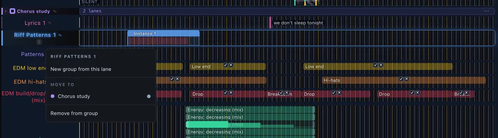The lane menu — start a band, move the lane into one, or take it back out.

4. Rename the band by clicking the pencil on its header, so it says what the lanes are for.
5. Collapse it with the chevron when you’re working elsewhere — the lanes fold away behind the header and nothing is deleted. The checkbox beside the name is the band’s own visibility: it turns every lane in the group off at once, and shows a dash when only some are on.
6. End it from the header’s ⋯ menu. Ungroup dissolves the band and keeps every lane; Delete group and its N lanes… takes the annotations with it, and asks first.

Groups are saved with the song’s annotations, so they come back when you reopen it. Detector lanes can’t join one (they’re rebuilt on every render), and bands only draw in the Annotator Tool — Dataprep and Algorithm Inspect leave out the header along with the lanes it covers.

Deep dive: Annotation Workspace and Keyboard Shortcuts.

Comparing algorithms

▶ Check the algorithms against your work

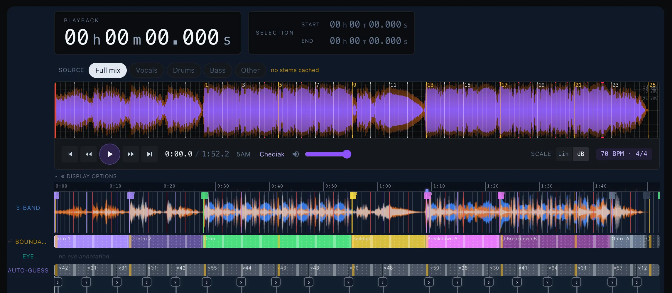Algorithm Inspect — each detector’s predictions stacked as colored timelines over the waveform, with your reference layers (Boundaries / Auto-guess) lined up beneath.

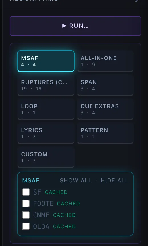Tick detectors in the right sidebar — grouped by family (MSAF, All-in-One, Ruptures/CPD, Span, Loop, Cue, Lyrics, Pattern, Custom). Every tick fires a run, cached by file hash, so repeats are instant.

The Evaluation tab — choose what to evaluate against, drag the tolerance slider τ, switch the Custom-eval options, and see the best / worst detector for this song at a glance.

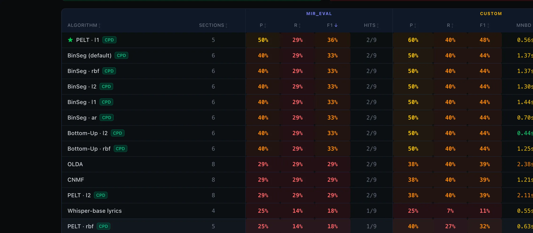Every detector ranked for this song — mir_eval precision / recall / F1 / hits, alongside the Custom engine’s MNBD and CSR columns.

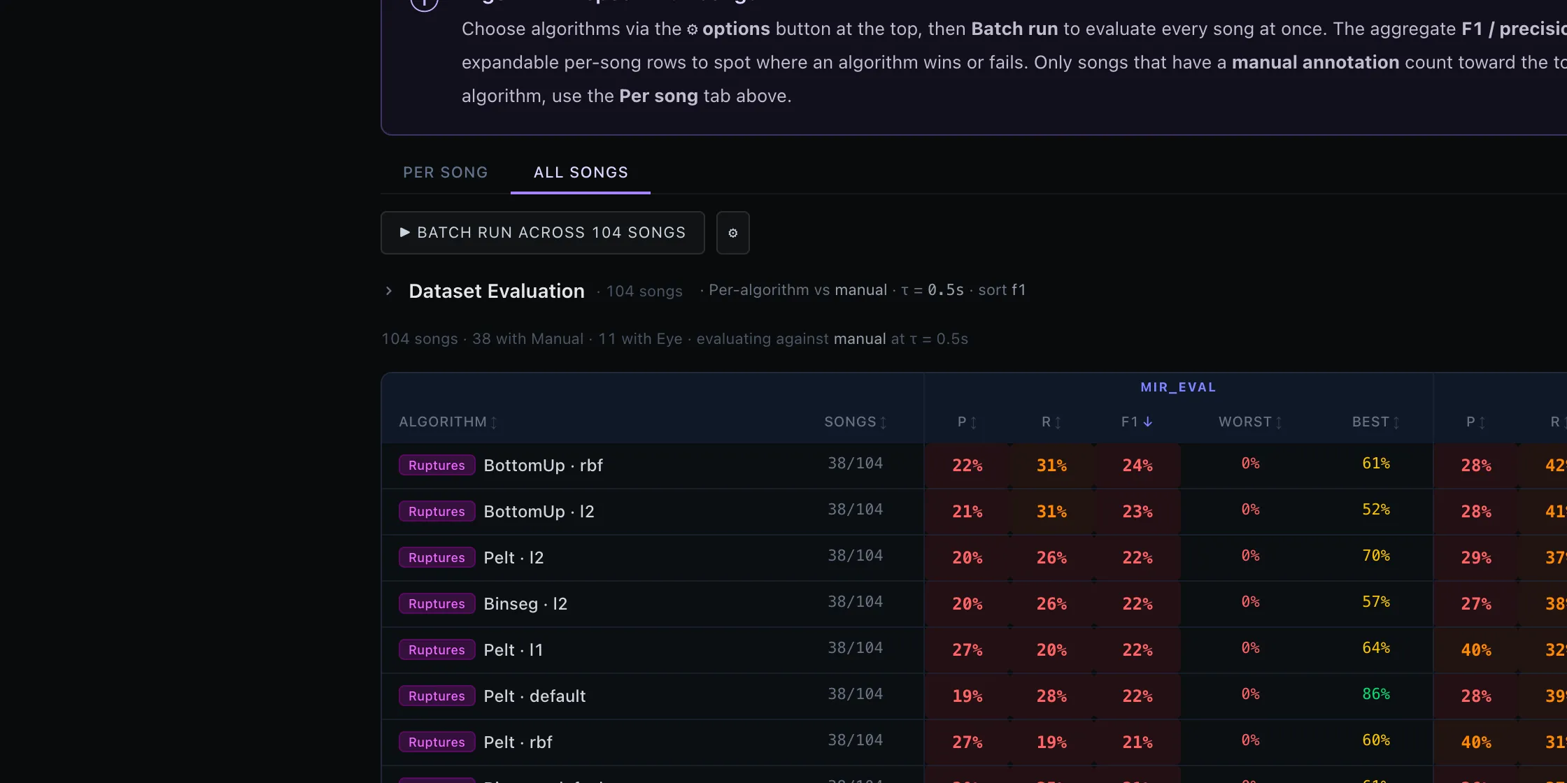The All songs tab — a dataset-wide leaderboard (here: 104 songs, 38 with a manual reference) you can re-sort by F1, precision, recall, MNBD, or CSR.

The whole point of TimeCues — line every detector up against your ground truth and see who wins, per song and across the corpus.

1. Have a reference layer. You need at least one of Manual or Auto-guess (reviewed) on the song to evaluate against. Without that, every metric is meaningless — F1 against an empty reference is undefined.
2. Switch to the Algorithm Inspect tab and pick a song from the sidebar.
3. Tick algorithms in the right sidebar. Each one you tick fires a detector run (cached by file hash, so a repeat run is instant). Their predictions stack as colored timelines underneath the waveform.
4. Pick a reference in the Reference dropdown — Manual or Auto-guess. The metrics panel below the canvas updates immediately.
5. Pick the evaluation engine:
   • mir_eval — the research-standard hit-rate / F1 / precision / recall computed by the mir_eval library. Use this when you want results that other papers can compare against.
   • Custom — adds Mean Nearest-Boundary Distance (MNBD, in seconds), Critical-Section Recall (CSR, restricted to ★-marked boundaries), candidate-aware matching (a boundary with multiple S-split candidates scores against whichever lands closest), and an optional-weight slider that lets you down-weight optional boundaries when computing F1.
6. Drag the tolerance slider (τ) to widen or narrow the matching window in seconds. Most published numbers use τ = 0.5 s or τ = 3 s.
7. Switch to the All songs sub-tab to batch-run the same selection across the whole corpus. The leaderboard sorts by F1 / precision / recall / MNBD / CSR — click a column header to re-sort. Each row expands to per-song scores so you can spot which songs an algorithm chokes on.
8. Pre-compute the cache in Dataprep first if you have many songs: the Run all algorithms button warms the cache for every detector × every song, so the batch view loads instantly later.

What you need: The default docker compose up stack covers MSAF, Ruptures, and the librosa / mir detectors — tick those with zero extra setup. All-In-One stays greyed out (“Demucs profile needed”) until the stack is up with --profile demucs-cpu or --profile demucs-gpu (local dev: pip install -r tools/requirements-allin1.txt). The experimental detectors (BeatNet, Silero-VAD, PANNs, …) need both the --profile experimental-models sidecars and their per-family toggle in Settings → Experimental annotation types & models — every experimental flag is off by default. Full map: Flags & compose profiles.

Deep dive: Inspect Workspace and Inspect All.

The Auto-guess workflow — consensus & clustering

Auto-guess lives alongside Manual under the Boundaries layer type.

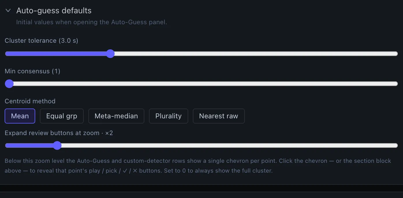Auto-guess defaults — cluster tolerance τ, minimum agreement count, and the source-detector subset that feeds the consensus.

Auto-guess is the fastest path from “I just dropped a song in” to “I have clean ground truth boundaries.” It runs 30+ detectors in parallel, clusters their boundary predictions in time, and lets you tick through the clusters one at a time with three keys: ✓ / ✗ / @. The output is a single, reviewed boundary layer.

The mental model

Think of it as wisdom of crowds for boundary detection. No single detector is reliable — librosa beat-based segmentation might miss a break, MSAF SF might fire on every snare fill, allin1 has its own priors. But if six different detectors all fire within 200 ms of each other, something is happening there. Auto-guess turns that agreement into a single candidate and asks you to confirm it.

Step by step

1. Lock BPM and grid in Dataprep first. Auto-guess clusters in seconds, but candidates are still snapped to the grid you set up.
2. Pre-compute the detector cache. From Dataprep, click Run all algorithms to warm the cache for every built-in detector on this song. (You can also do it from Algorithm Inspect — the cache is shared.) Auto-guess won’t run until the source detectors have results to consume.
3. Switch to the Annotator Tool → Boundaries → Auto-guess tab.
4. Click Generate AutoGuess. The server pulls every cached detector’s output, clusters all the boundary times into groups within a cluster tolerance τ (default 3 s, slider exposes 0.5 s – 10 s), and returns one candidate per cluster. Each candidate carries:
   • a timestamp (the cluster centroid, weighted by detector confidence when available);
   • an agreement score — how many of the 30+ detectors fired inside this cluster;
   • the list of contributing detectors so you can see who agrees.
5. Tick through the candidates with J / K (next / previous). At each candidate, press:
   • ✓ (or A for accept) — the candidate becomes a confirmed boundary in your Auto-guess layer.
   • ✗ (or R for reject) — the candidate is dropped. Use this for false positives: a swell that no human would call a section boundary, a snare fill that fooled three detectors, an outro fade-out that everyone agreed on but doesn’t actually mark a transition.
   • @ (or E for edit) — accept the candidate but nudge it in time before committing. Use this when the consensus is in the right neighborhood but the cluster centroid landed half a bar early.
6. Adjust the cluster tolerance if you’re seeing too many candidates (lower τ) or too few (raise τ). Regenerating with a different τ is cheap — the per-detector cache is already warm, only the clustering re-runs.
7. Flip the layer to reviewed when you’ve ticked through every candidate. The Auto-guess layer is now eligible as a reference in Algorithm Inspect — meaning you can train new detectors against the boundaries the consensus revealed.

Why this is faster than annotating from scratch

A typical 3-minute song has ~8–12 section boundaries. From scratch you play the song through, drop M boundaries, then go back and refine each one — usually 10–15 minutes per song. With Auto-guess, the consensus typically surfaces ~80–90% of the true boundaries on the first pass, plus a handful of false positives. Ticking through 12 candidates (✓ ✓ ✗ ✓ @ ✓ …) takes 60–90 seconds. The remaining 1–2 missed boundaries you add by hand using normal Manual workflow.

Tuning the consensus

The AutoGuess grid search in Inspect All lets you sweep the clustering parameters across your whole corpus to find the F1-optimal tolerance and agreement-threshold settings. Use it once on a small labeled subset, then apply the winning parameters to the rest of the corpus.

What feeds the consensus: Auto-guess clusters whatever detectors have cached output, so the pool depends on what’s running. The default stack’s detectors are always in; All-In-One joins only when a Demucs profile is up, and the experimental families only when --profile experimental-models is running and their flag is on (default off). More detectors → stronger agreement, so warm the cache with Run all algorithms first. See Flags & compose profiles.

Deep dive: Auto-Guess Internals covers the full clustering algorithm, the per-detector confidence weighting, and the exact grid-search procedure.

Writing a custom detector

▶ Write your own algorithm in the Playground

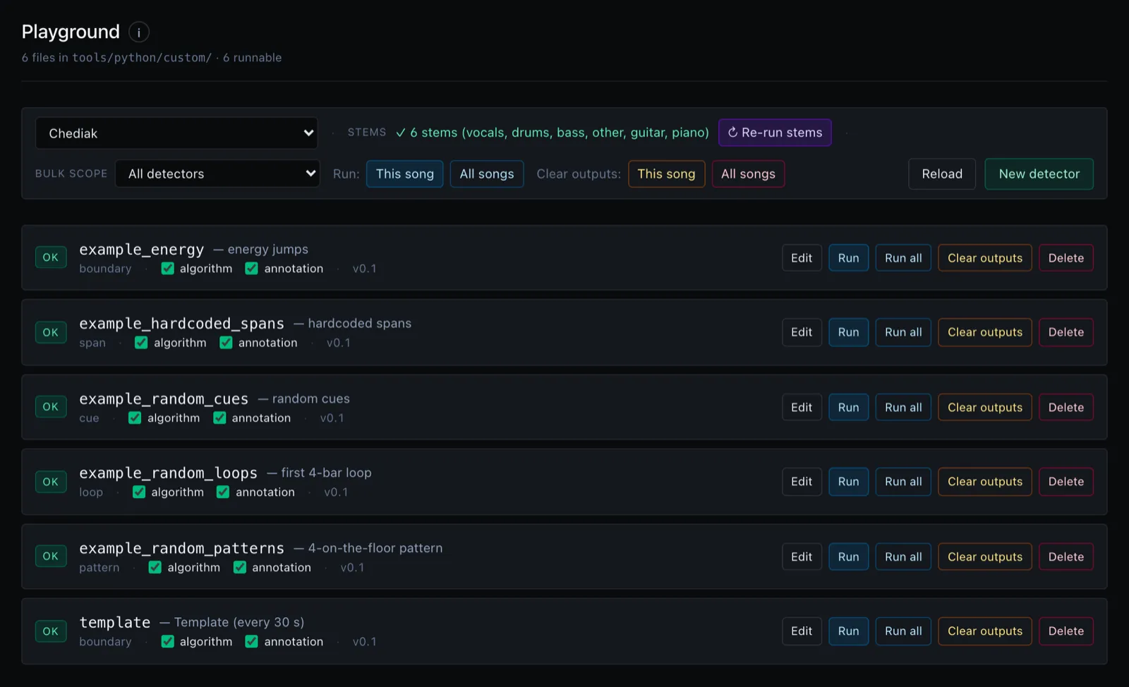The Playground — write, save, run, and inspect custom Python detectors against the corpus.

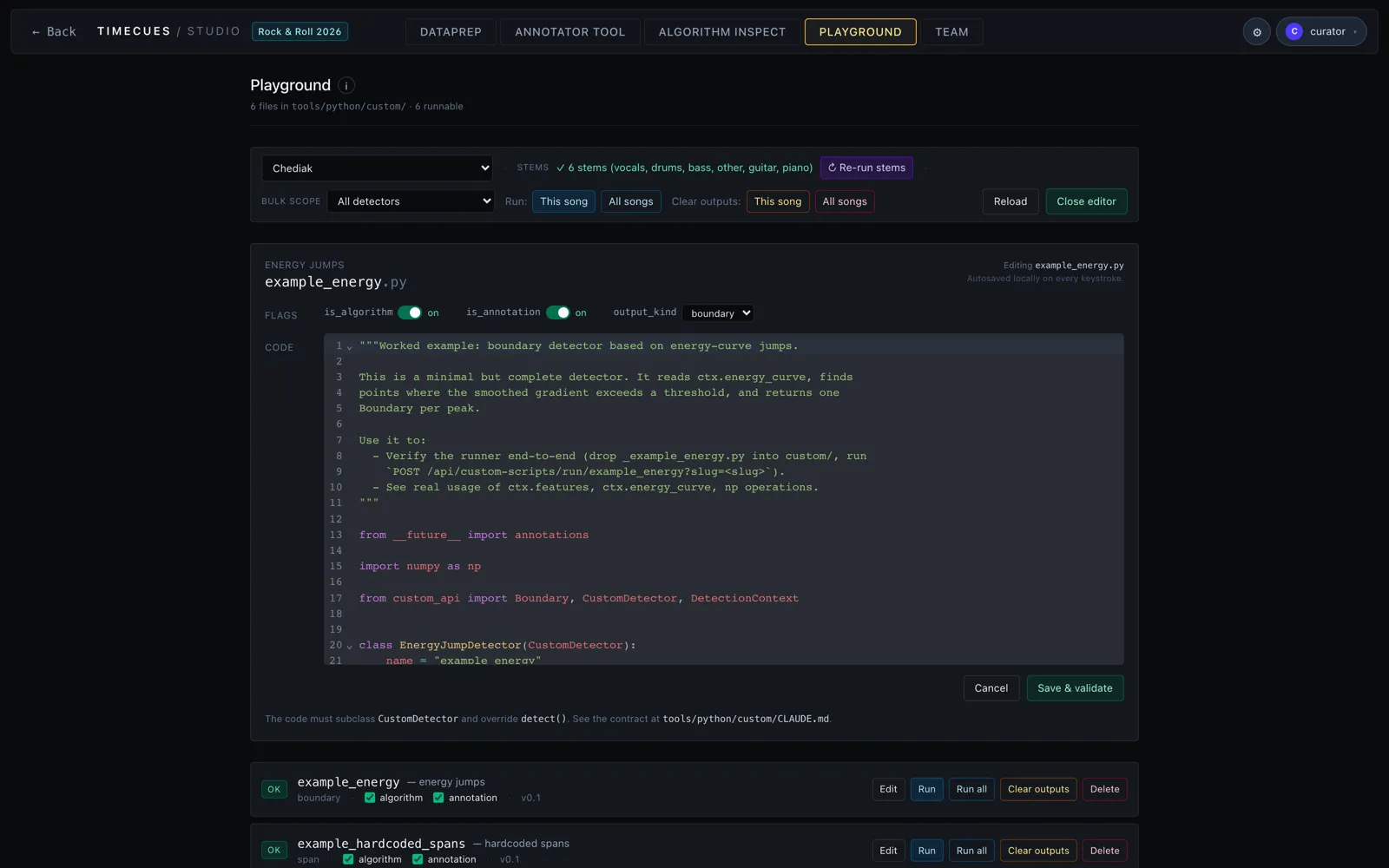Edit the detector source and manifest, then run it inline without a build step.

Each detector row — status, name, kind/version, and Edit / Run / Run all / Clear outputs / Delete.

Drop a Python file in tools/python/custom/, reload, and your algorithm shows up as an overlay alongside every built-in detector.

1. Switch to the Playground tab. Hidden in Demo Mode.
2. Write a .py file that exposes a function matching the detector contract — the Custom Detectors section of the user guide has the exact signature. Roughly:

   def detect(audio, sr, **kwargs):
       """Return a list of Boundary objects (time + label)."""
       boundaries = my_segmentation(audio, sr)
       return [Boundary(time=t, label=lbl) for t, lbl in boundaries]

3. Upload it via the Playground UI’s file picker (or drop it into tools/python/custom/ on disk and click Reload). The registry hot-reloads and the new detector appears alongside built-ins in Algorithm Inspect, Auto-guess’s source pool, and the Dataprep batch-run picker.
4. Run it on a song in Algorithm Inspect and check the overlay.
5. Iterate — edit the script, re-upload (or just re-save and Reload), re-run. Cached results are keyed by the script’s file hash, so a tweaked script always produces a fresh run; reverting to a previous version transparently re-hits the cache.

What you need: Nothing extra — the custom sidecar (:8005) ships in the default stack, so custom detectors run without any profile. Scripts are read from CUSTOM_SCRIPTS_DIR (default ./tools/python/custom); set it to a persistent path in .env for production. The Playground tab is hidden in Demo Mode — sign in to a claimed corpus to see it. Any Python package your detector imports must be installed in the custom sidecar’s environment (rebuild its image, or pip install it on the ./run.sh host).

Deep dive: Custom Detectors documents the full Python contract, the parameter schema for the UI, and how cached results are stored.

Multi-annotator: comparing two people’s work

▶ Compare two annotators’ work

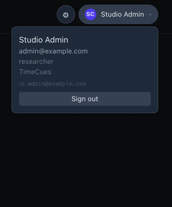Each sign-in is a distinct annotator id, so two people’s manual layers never clobber each other.

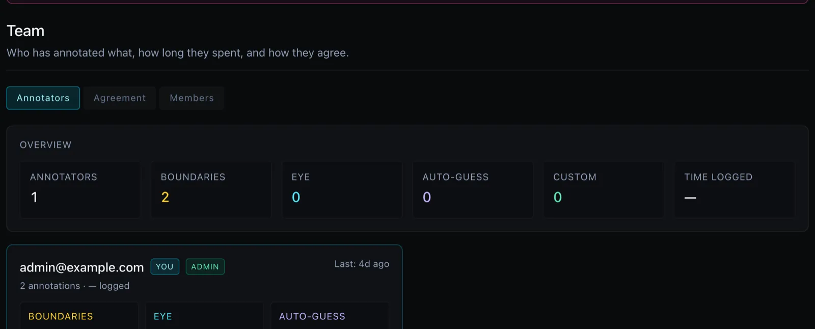The Team dashboard — per-annotator boundary and auto-guess progress at a glance.

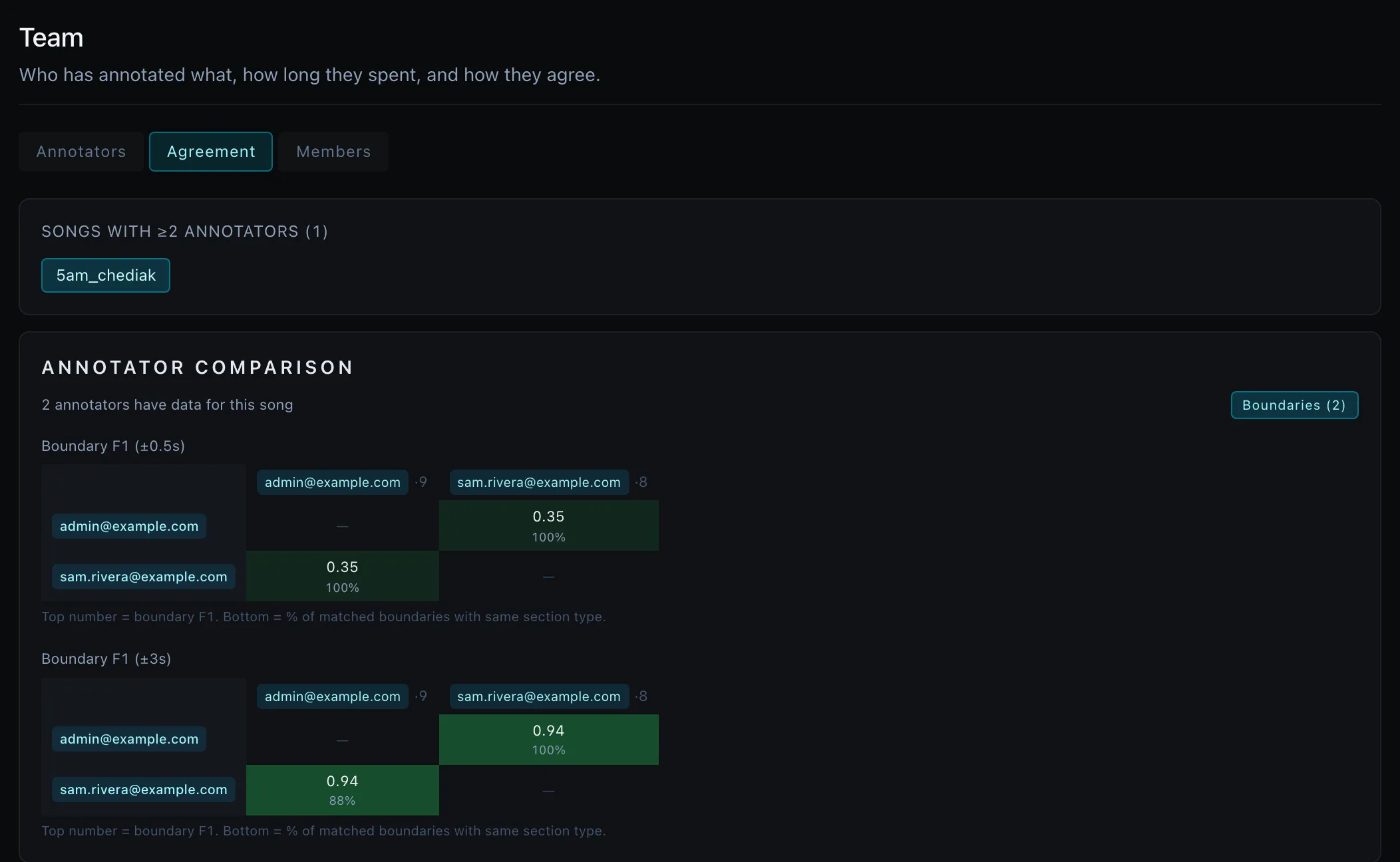Inter-annotator agreement — where two people’s boundaries pair up within τ, and where they disagree.

The per-annotator namespace is what keeps two people’s manual annotations from clobbering each other; the Compare sub-tab is where you put them side by side and resolve disagreements.

1. Sign in with two different accounts (two browsers, or one browser with a private window). Each becomes a distinct annotator id; annotations land at data/annotations/<layer>/<annotator-id>/<slug>.json.
2. Each annotator does a Manual pass on the same song.
3. Open the Annotator Tool’s Compare sub-tab while signed in as an admin or researcher (regular team annotators only see their own work).
4. Pick the two annotators in the Compare picker. Their layers render as two stacked timelines on the waveform, in distinct colors.
5. Per-boundary diff readout appears in the panel below — every boundary that’s within τ of a peer is paired, everything else is flagged as a disagreement.
6. Adjudicate by switching to either annotator’s layer (top-right View as dropdown) and editing — or use the Team page’s “Merge into Auto-guess” action to fold both annotators’ boundaries into a shared Auto-guess layer that you can then review together.

What you need: Real sign-in. Demo Mode is single-user (everything lives in localStorage), so it has no separate annotator namespaces. Google sign-in works out of the box on localhost via the VITE_GOOGLE_CLIENT_ID shipped in docker-compose.yml; on any other hostname set your own client ID in .env and add the origin to its Authorized JavaScript origins. The Compare sub-tab is admin / researcher only.

Deep dive: Sign-In & Identity and Team Dashboard.

The other model: one shared annotation, one editor at a time

Everything above assumes two readings worth comparing. When the goal is a single ground truth instead, make the song collaborative: the team edits one annotation, and takes turns.

Collaboration is per song. A collaborative song opens read-only for everyone; you press Lock to edit to take it and Unlock to hand it back, and a bar above the annotation panel always names who holds it — whether they are actively editing, holding it quietly, or whether their tab has stopped answering. Nothing unlocks on a timer: taking a song from someone is always a deliberate act, and their work is saved as a version before it moves.

Every hand-off is a version you can read and restore, so “put it back the way Alice had it” is a button rather than an archaeology project.

Pick per song: Compare for independent readings you want to measure against each other, collaborative for one annotation the team converges on.

Deep dive: Collaborative songs.

BPM auto-detection chips

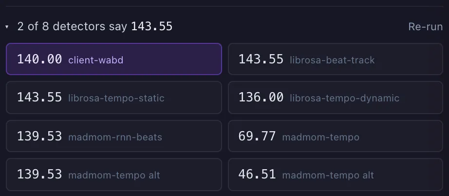The AUTO-DETECTED row — click a chip to adopt that detector’s BPM; Re-run forces a fresh pass.

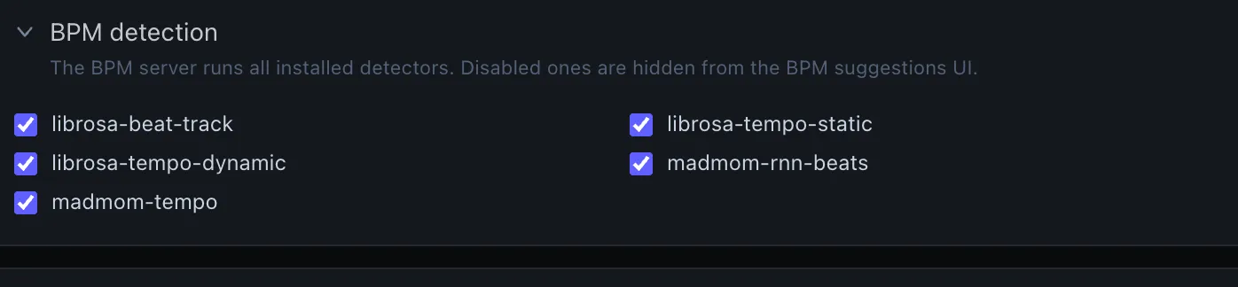Choose which detectors appear in the chip row under Settings → Research → BPM detection.

Five detectors race in parallel; you click the chip whose number matches what you hear, and the song’s BPM is set.

1. In Dataprep, open step ① Tempo in the Song setup sidebar.
2. A row of Auto-detected chips appears just below the BPM input. As detectors finish, their chips light up:
   • client-wabd — runs in your browser via web-audio-beat-detector the moment the audio decodes. Fastest, typically the first chip to appear.
   • librosa-beat-track — onset → beat tracking from librosa.
   • librosa-tempo-static — librosa’s global tempo estimate.
   • librosa-tempo-dynamic — librosa’s frame-wise tempo (dominant mode reported).
   • madmom-rnn-beats — RNN beat tracker from the CPJKU madmom fork.
   • madmom-tempo — madmom tempo histogram.
3. Click a chip to adopt its BPM into the input. Click another chip to switch.
4. Disagree on the octave? Halve or double the value in the input manually — many detectors confuse half-time and double-time. The metronome panel below is the fastest way to verify: play the song with the metronome on and listen for the click to land on the kick.
5. Click ↻ Re-run at the right of the chip row to force a fresh detection (ignores the cache). Useful after replacing the audio file.
6. Filter which detectors appear under Settings → BPM Detection — turn off detectors that are slow or that you don’t trust on your corpus.

What you need: Nothing extra — the five server-side detectors all live in the bpm sidecar (:8004), part of the default stack, and client-wabd runs entirely in your browser. No profile, no model download. Every detector is enabled by default; switch individual ones off under Settings → Research → BPM detection.

Deep dive: Song Info Bar → BPM.

Aligning the beat grid

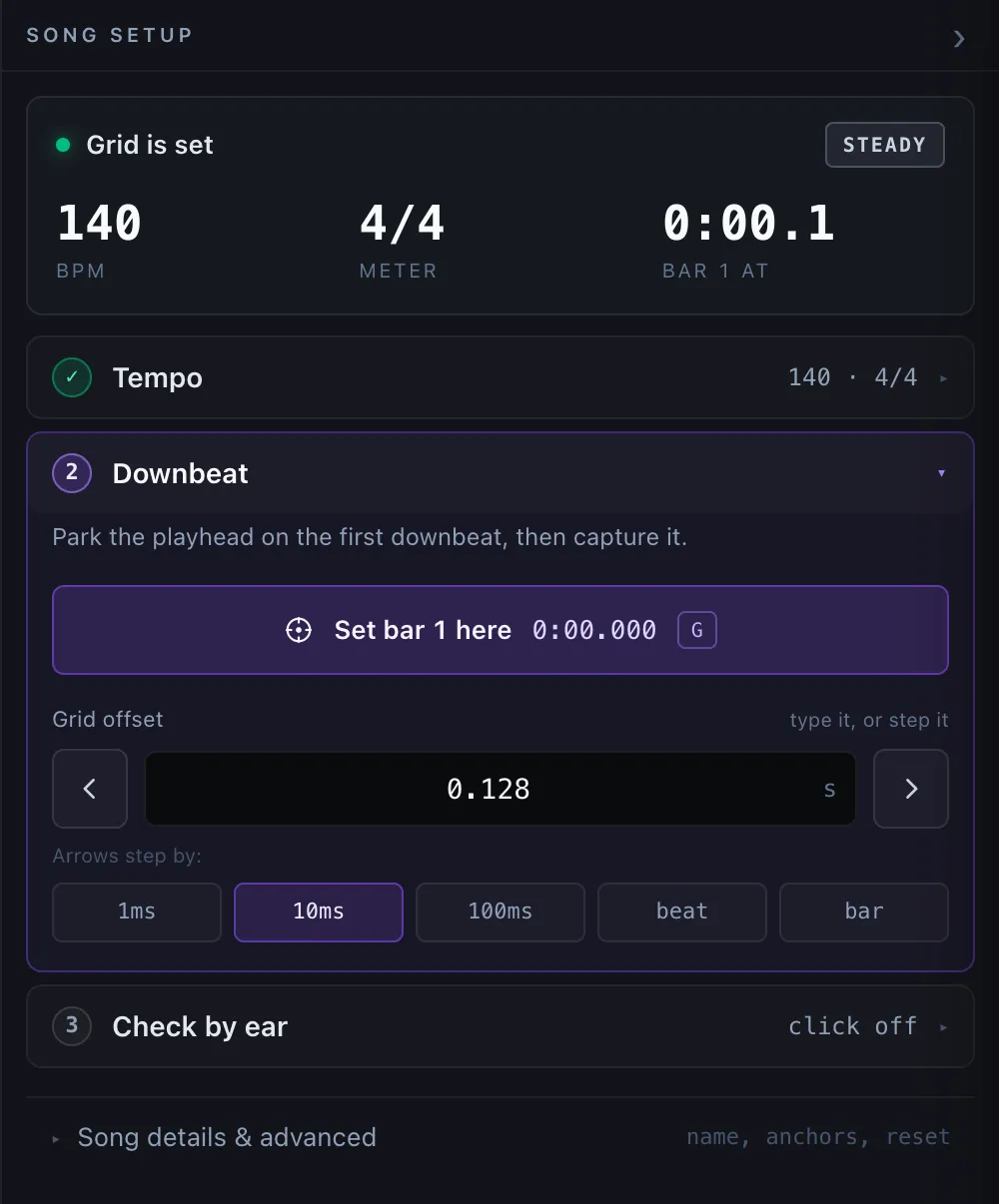The Tempo panel in Dataset Prep — set the BPM, then anchor bar 1 with Set bar start (G), Nudge, and the Grid offset (s) field.

Turn on Show beat grid and the lines ride on the audio — white for beats, red for bar downbeats, and the yellow marker for your bar-start anchor (beat 1). Aligning means sliding those red bar lines onto the song’s real downbeats.

Tempo mode — Steady, Mapped, or Hand-placed; only the active mode’s grid is drawn downstream.

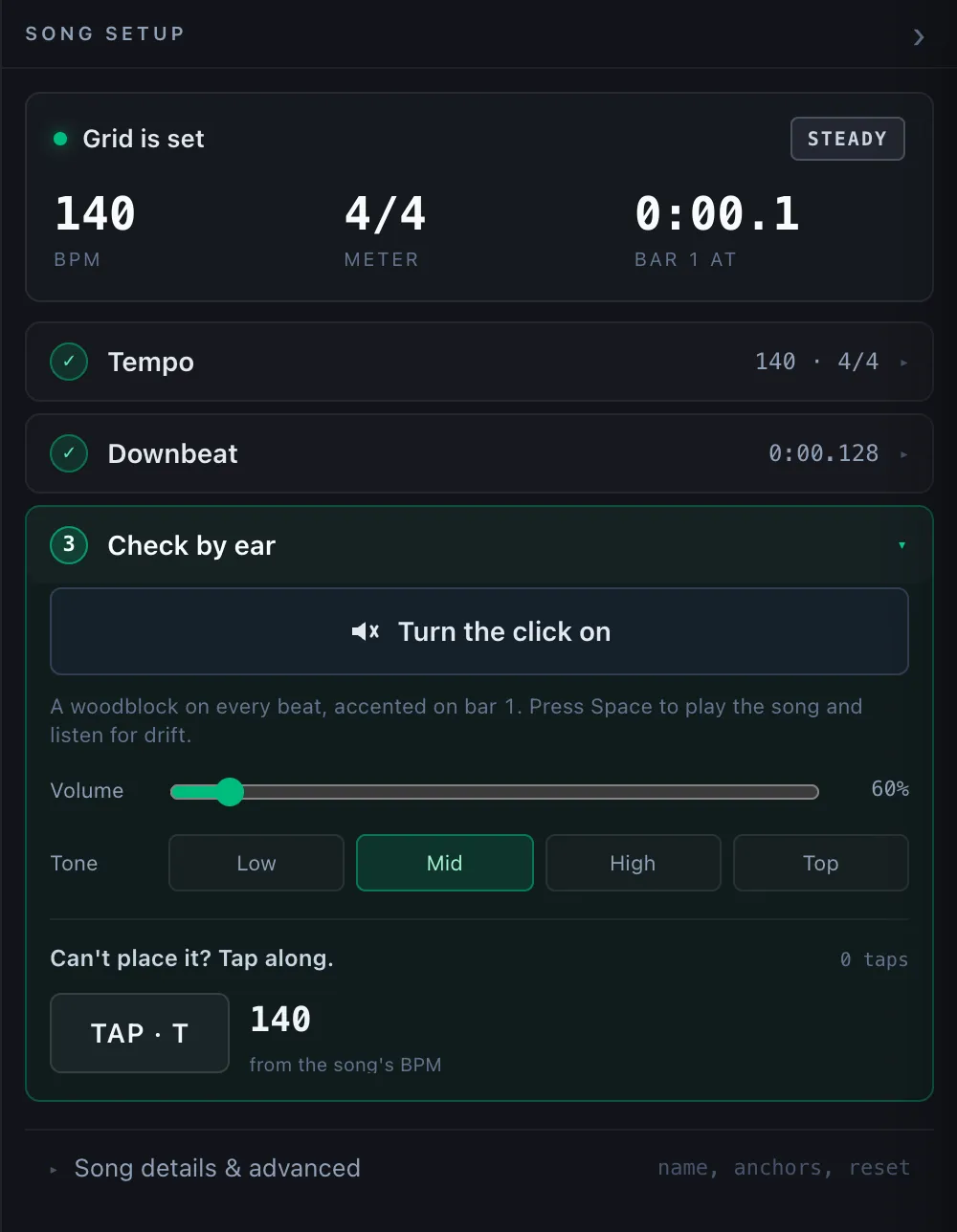Verify the grid with the metronome — the click should land on the kick, not before or after.

BPM tells the app the tempo, but not where bar 1 starts. Without an anchor every snap lands on the closest grid line — which may be one or two beats off the song’s actual downbeat. Aligning the grid takes ten seconds per song and prevents an entire category of annotation drift.

Why this matters

Every Manual boundary snaps to the song’s beat grid when Snap is on (which is the default — see Snap toggle). If your grid is misaligned by 240 ms, every boundary you drop with M lands 240 ms early. Then when you compare against algorithm output they look “always slightly off” — and that’s the grid’s fault, not the algorithm’s. Catching this in Dataprep saves debugging in Algorithm Inspect later.

The grid-readiness glyph

Each song row in the sidebar carries a ♩ glyph that summarizes how ready that song is for annotation:

• 🔴 red ♩ — no BPM set. Annotator Tool won’t open.
• 🟡 amber ♩ — BPM is set but the bar start has not been confirmed. Annotation will work, but every boundary’s snap may be one beat off the actual downbeat.
• 🟢 emerald ♩ — BPM set and bar start anchored. Safe to annotate.

The goal of the alignment workflow below is to get every song to emerald before you start annotating.

Step by step

1. In Dataprep, pick the song in the sidebar. The viz canvas loads, the audio decodes, the waveform draws.
2. Open step ① Tempo in the Song setup sidebar if it’s collapsed.
3. Set BPM first — click an Auto-detected chip or type a value. See BPM auto-detection chips above for the chip-by-chip details. The grid overlay on the waveform appears as soon as BPM is non-zero.
4. Listen for the first kick of the song’s actual content (usually right after the intro / pickup). Press space to play, pause when you hear it.
5. Press G at the playhead to set the bar start. The grid overlay snaps so that beat is now beat 1 of bar 1. The sidebar glyph flips from amber ♩ to emerald ♩.
6. Verify with the metronome. Open step ③ Check by ear, click Turn the click on, and press space. You should hear the click land on the kick, not slightly before or after. If the click drifts: go back to step ② Downbeat and step the offset until it locks. If the drift grows across the song rather than staying constant, the tempo itself is wrong — fix the BPM in step ①, or split the grid where the feel changes in Mapped.

Grid Offset — the fine-tuning slider

Below the BPM input is a Grid Offset field, in seconds, range ≥ 0, step 0.001. This is where the grid’s bar-1 boundary sits relative to t = 0 in the audio. Setting bar start with G auto-fills it; you can also type a value directly if you’re matching to an existing JAMS/REAPER reference.

When to nudge Grid Offset by hand:

• Audio file has a long silence at the start — the first kick is 3 seconds in, but the producer intended bar 1 to be at exactly 3.000 s. Type that.
• Imported from another tool — the JAMS file says bar_offset = 1.2375. Type that.
• The G placement is off by a few milliseconds — you anchored near the kick but not exactly on it. Nudge ± 10 ms at a time and re-verify with the metronome.

The three tempo modes

A segmented control at the top of step ① Tempo tells the app how the grid is laid out across the song:

Mode	When to pick	What it does
Steady (default)	DAW-produced music, EDM, hip-hop — anything with a click track at the source.	One BPM number, one bar-start anchor, one rigid grid for the whole song. The fastest and most precise.
Mapped	A song whose count restarts partway through — a meter change, a splice, a free intro before the band enters.	A tempo map. You place markers, and each one starts a new bar 1 with its own tempo and its own time signature; the bar the previous grid was mid-way through is cut where the marker lands.
Hand-placed	The last stubborn stretch of an otherwise fine song, and audio with no steady pulse to find at all — rubato playing, a passage with no drums, spoken word, field recordings.	Pinned beats on top of a base grid you pick when you enter the mode. Everything you don’t pin keeps following the base.

Steady handles ~95% of recorded music. The modes stack rather than compete: Hand-placed sits on top of whichever of the other two you give it as a base, so a song with one loose bridge is normally Steady with a few pinned beats, not a song hand-placed from scratch.

Common pitfalls

• Anchoring on the pickup, not the downbeat. Many songs begin with a pickup beat (a single drum hit or guitar strum before bar 1 proper). Anchoring on that puts bar 1 a beat early. Listen for the full kick + snare pattern to know you’re on the real downbeat.
• Songs that drift but you stay in Steady mode. The metronome starts on the kick at second 0 but is off by half a beat at second 120. TimeCues has no mode that follows a drummer’s natural drift automatically — a Drifting mode existed and was removed, because its anchors came from a tempo detector, which made any annotation snapped to them partly a detector’s opinion rather than ground truth. Set the BPM that fits the bulk of the song, then reach for Mapped (a marker where the feel changes) or Hand-placed (pins on the beats that wandered).
• BPM is half what it should be. Many detectors report half-time for songs with strong off-beat snare patterns. Double the BPM manually and re-anchor; the metronome will tell you instantly if you guessed wrong.
• Audio file has been re-encoded and the start timestamp moved. Re-anchor; old Grid Offset values are stale.

What you need: Just the default stack — BPM detection (the bpm sidecar, :8004) is always on, and all three tempo modes (Steady / Mapped / Hand-placed) are core features with no flag to enable and nothing extra to install.

Deep dive: Song Info Bar → BPM, Grid Offset, Grid Mode (Steady · Mapped · Hand-placed), Which mode does this song need?, and Metronome Panel.

Mapped and hand-placed tempo

Steady assumes one tempo, and one count, for the whole song. That covers most produced music. Two things break it: a song whose count restarts partway through — a meter change, a splice, a free intro before the band enters — and audio with no steady pulse to find at all. Mapped and Hand-placed are how you make the grid follow the music instead of fighting it.

Both live in the same ① Tempo step as Steady, behind the three-way mode picker. Switching modes is non-destructive — each mode keeps its own grid data, and only the active mode’s grid is drawn downstream in the Annotator Tool and Algorithm Inspect.

Mapped — a tempo map, one bar 1 per segment

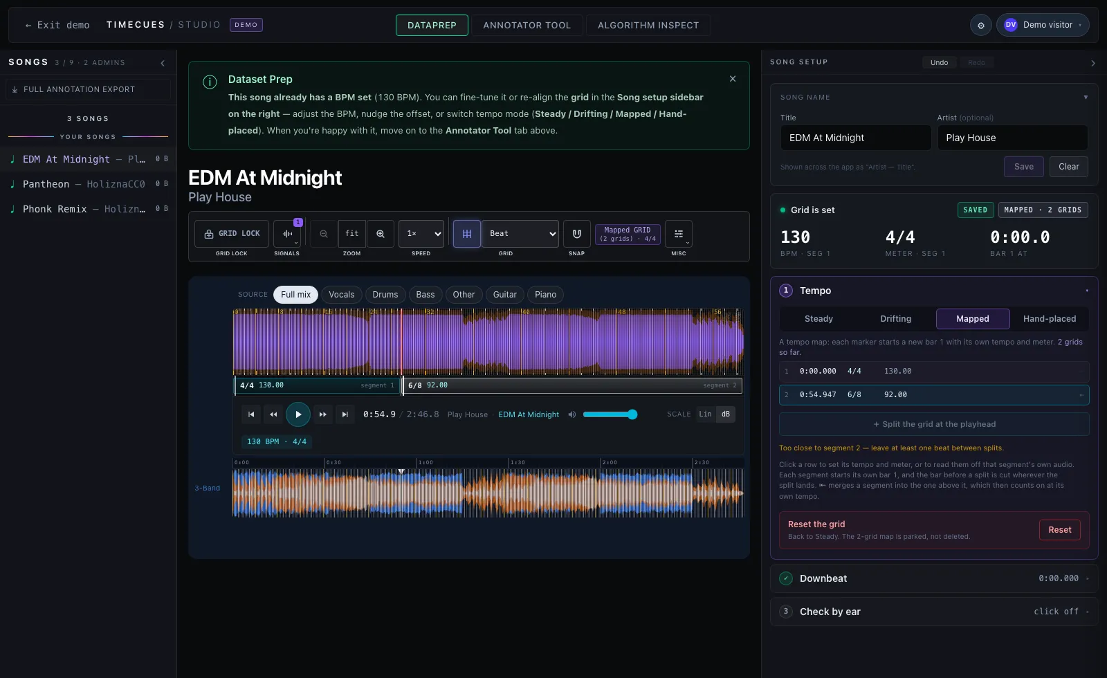Mapped mode — the tempo-map list under the mode picker, and the segment lane under the waveform: two grids (4/4 at 130, then 6/8 at 92), the double-bar-line marker between them, and the hatched cut bar just before it.

Mapped represents the song as a tempo map: a row of segments that tile the track end to end, each carrying its own start, its own BPM and its own time signature. A marker doesn’t bend the grid — it starts a new bar 1, and the bar the previous grid was in the middle of is cut where the marker lands.

1. Switch to the Mapped tab. The song-level BPM field and meter chips disappear, because in Mapped the tempo belongs to the segments.
2. Park the playhead where the count restarts and click ＋ Split the grid at the playhead. Everything after the marker counts from a fresh bar 1.
3. Give the segment its tempo and meter from its row in the list — or let it find its own.

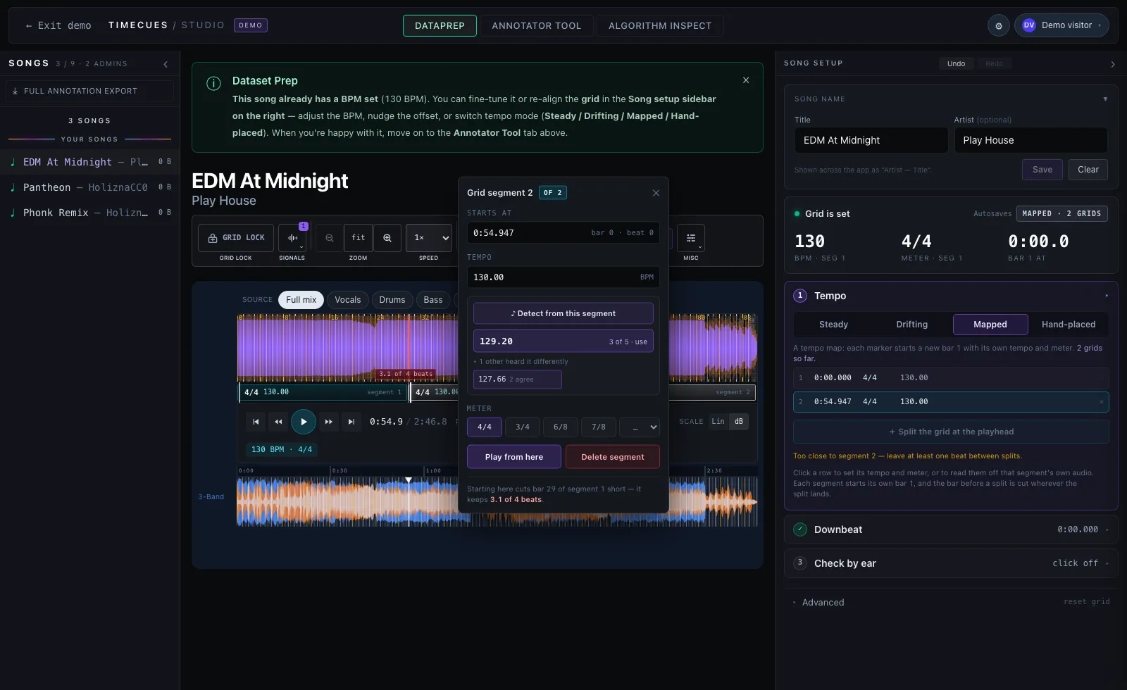A segment can detect its tempo from its own audio: the detectors are fed only the span between this head and the next, so a slow intro doesn’t drag the estimate for the rest of the track.

4. Merge two segments by right-clicking a head on the lane, using the ⇤ at the end of a row, or clicking ⇤ Merge with previous. The head goes and the segment on its left grows to swallow the span, counting on at its own tempo and meter — which is why the button names the surviving tempo in its tooltip. Segment 1 has nothing before it, so it can never be merged away.

What a split does and doesn’t move. It rewrites the ruler, not the data. Every cue, span and loop keeps the absolute time it was placed at; only the bar.beat label that time resolves to changes. Because that renumbers bars downstream, adding or moving a segment counts as a grid change and raises the usual Grid Lock prompt on songs that already carry annotations.

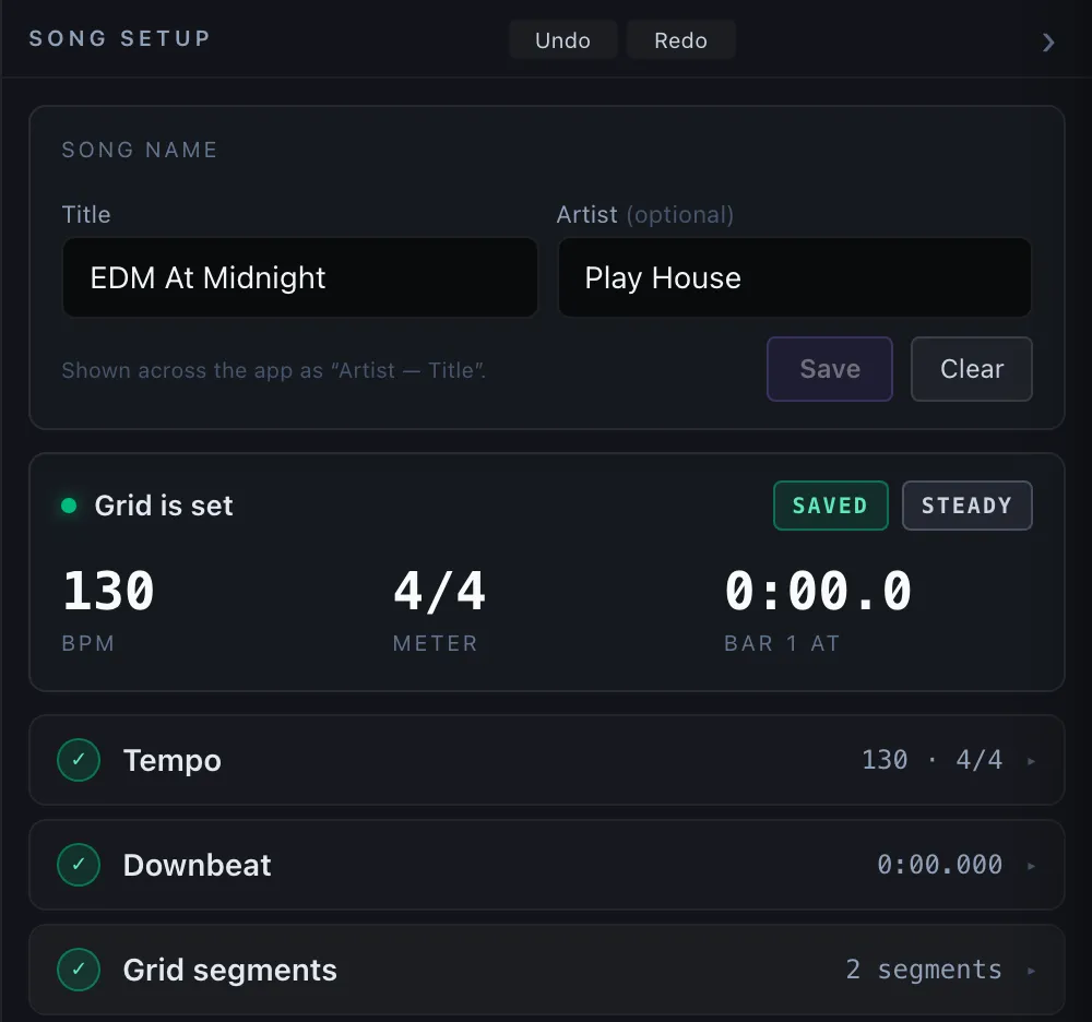Grid edits are undoable — Undo and Redo sit in the Song setup sidebar header, and ⌘Z brings a dropped split back.

Hand-placed — pin beats by hand

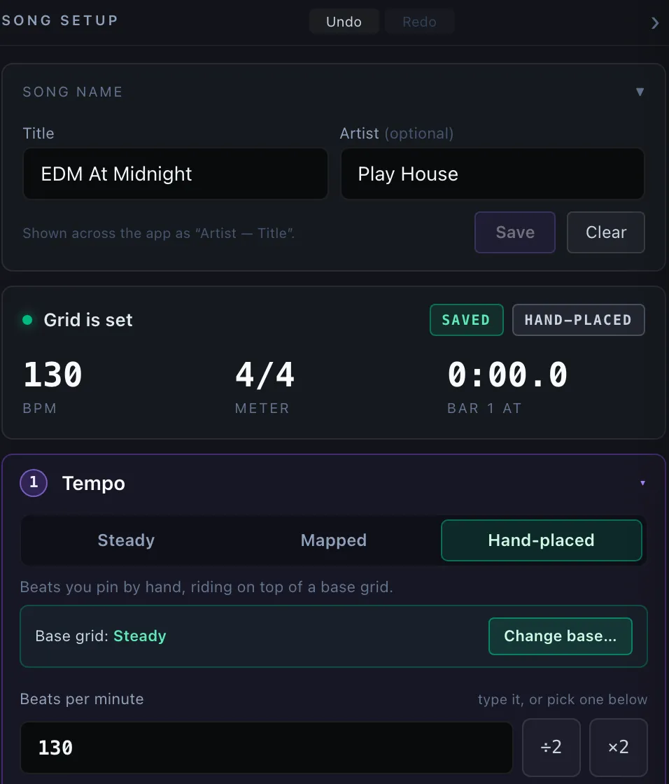Hand-placed — per-beat pinning on top of a base grid, with the reset controls.

Hand-placed is a two-layer system: a base grid plus pinned beats you place by hand on top of it. Use it for the hard cases — rubato playing, a section that deliberately slows at the end, a passage with no drums, spoken word and field recordings, and the last stubborn stretch of a song that is otherwise fine.

1. Switch to the Hand-placed tab. A modal asks you to pick the base grid: Steady (pinned beats ride a single-tempo grid) or Mapped (they ride a grid that restarts bar 1 at each marker — greyed out until the song has a map). Esc or ✕ aborts, reverting to whichever grid you were on.
2. Pin beats on the waveform. Drag any beat line to where that beat actually lands; it becomes a pinned beat. Right-click one to unpin it. Everything you don’t pin keeps following the base.
3. Change the base later with Change base… under the picker. Pinned beats survive a base switch — only their drift against the grid underneath changes.
4. Wipe every adjustment with the reset at the foot of step ① Tempo. It renders only when there is something to undo, and the confirm names exactly what it will discard.

When to use which: stay on Steady for ~95% of recorded music; reach for Mapped when the song’s count restarts; reach for Hand-placed when there is no steady pulse to follow, or when a handful of beats refuse to line up. It is the most expensive mode — every pinned beat is a decision you make by hand — so reach for it after the other two have been tried.

What you need: Nothing extra — all three modes are core features in the default stack, with no flag to enable and nothing to install.

Deep dive: Grid Mode (Steady · Mapped · Hand-placed), Grid Segments — the Mapped mode’s tempo map, and Manual mode is a two-layer system.

Stem separation with Demucs

▶ Separate a song into stems

Pick a stem — Vocals, Drums, Bass, or Other — from the Source picker in the top viz bar.

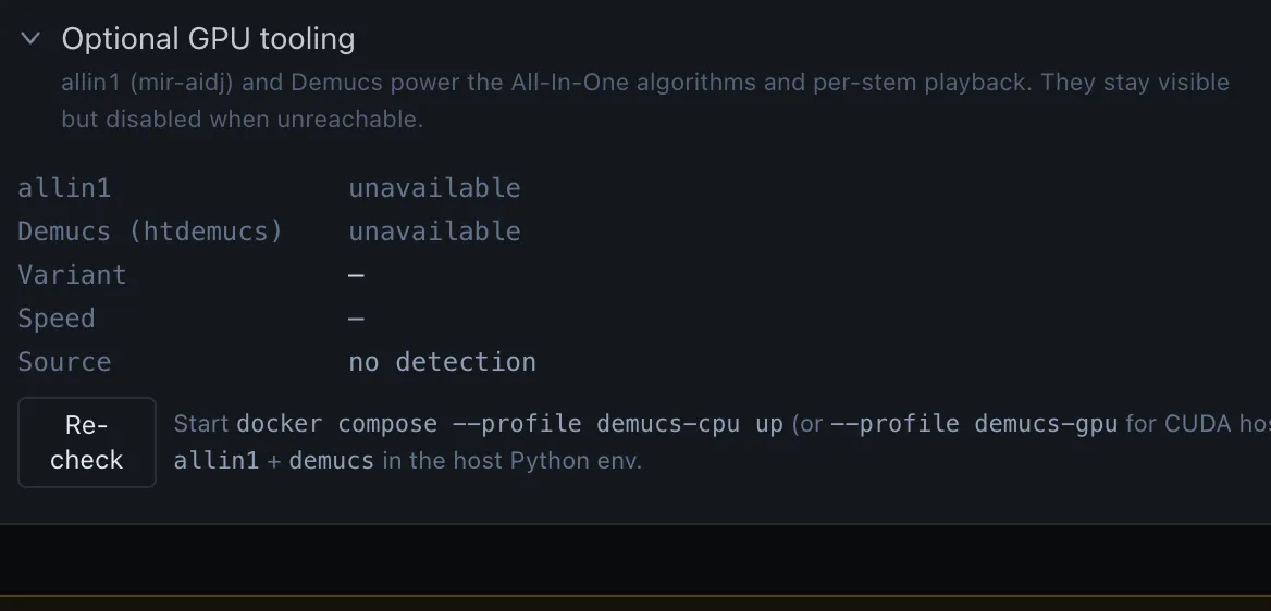Optional GPU tooling — the allin1 and Demucs install and acceleration status, set at compose time.

Four stem tracks (vocals / drums / bass / other) extracted by Demucs, available everywhere a source picker is shown.

1. Open the Source picker in the top viz bar — the dropdown next to the waveform mode chooser.
2. Pick a stem — Vocals, Drums, Bass, or Other. If stems aren’t cached yet for this song, Algorithm Inspect / Annotator Tool will show a “Stems not extracted” hint and (for admins) a Run Demucs button.
3. Admin: click Run Demucs to trigger the stems daemon on :8006. The daemon is not in the default stack — it only exists when you brought the stack up with a Demucs compose profile (--profile demucs-cpu or --profile demucs-gpu; see Flags & compose profiles). With no Demucs profile the ▶ Stem this song button is hidden entirely. Extraction takes roughly 3–5 minutes per song on the CPU profile and ~30–60 s on the GPU profile. Progress is streamed to the browser console; a failure raises a visible alert rather than silently swallowing (fixed 2026-05-20).
4. Once stems exist, switching between them in the Source picker is instant — the waveform redraws, the spectrogram re-renders, and every algorithm overlay re-evaluates against the chosen stem.
5. Useful in practice: running beat detection on the Drums stem alone often beats running it on the full mix; running boundary detection on Vocals surfaces verse / chorus transitions that the full-mix detector smears over.

Demo Mode ships with pre-extracted stems for the three sample songs (edm-at-midnight, pantheon, phonk-remix) — switching stems in demo is instant and does not run Demucs.

Deep dive: Stems server and Storage clear scopes.

Self-hosting on your own server

▶ Self-host TimeCues on your own server

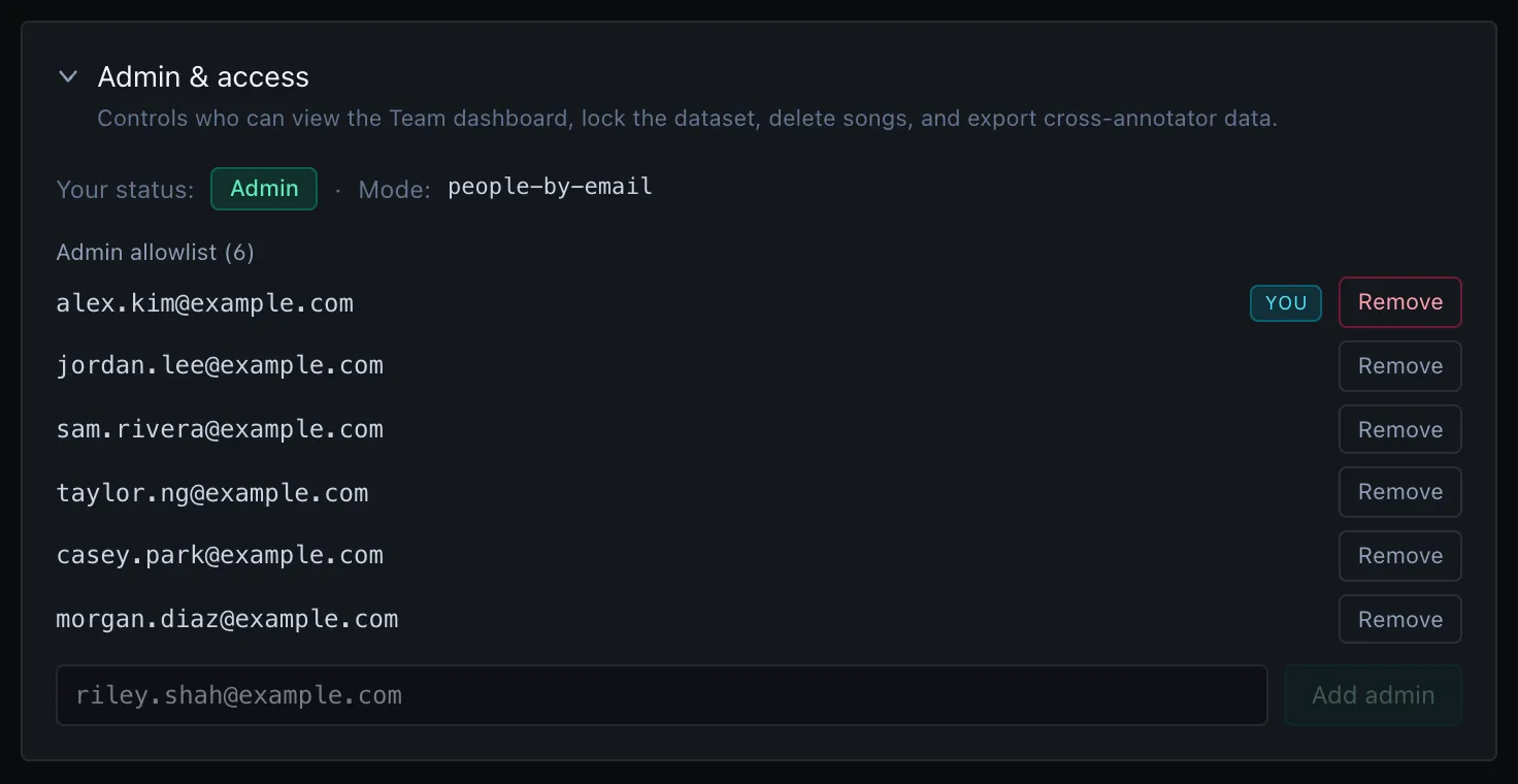Once the stack is up, the first sign-in claims admin — then manage the team from Settings → Corpus management → Admin & access.

The Docker Compose stack runs anywhere Docker (plus Compose v2) runs — a cloud VM, a homelab, or bare metal.

1. Clone the repo on the host and copy .env.example to .env. The defaults work for localhost as-is; the only flag you usually touch here is VITE_GOOGLE_CLIENT_ID (point sign-in at your own OAuth client) and, on a public host, DATA_DIR (a persistent disk, not the OS root). Full list under Flags & compose profiles.

2. Bring up the minimal stack — docker compose up --build starts the web app on :5173 plus six lightweight analysis sidecars: mir-eval (:8001), msaf (:8002), ruptures (:8003), bpm (:8004), custom (:8005), and mir (:8007). Stem separation and the experimental detectors are opt-in profiles — they do not start here (see step 5).

3. Put an HTTPS reverse proxy in front (Caddy, Traefik, or nginx + certbot) pointing at web:5173, so sign-in and the app work over TLS on your public hostname. Remember to add that hostname to your OAuth client’s Authorized JavaScript origins, or Google rejects the sign-in iframe.

4. First sign-in claims admin. Open the deployed URL, click Start a new dataset, sign in with Google. You’re now the first admin; invite the rest of your team from the Team page.

5. Optional heavy profiles (additive — combine freely):

   • --profile demucs-cpu — stem separation + All-In-One, works on any host, ~3–5 min/song.
   • --profile demucs-gpu — same features, CUDA-accelerated (~30–60 s/song), needs an NVIDIA GPU and is amd64-only.
   • --profile experimental-models — the eight Phase-1+ MIR detector sidecars (BeatNet, Silero-VAD, Whisper, …).

   e.g. docker compose --profile demucs-cpu --profile experimental-models up -d --build matches the hosted instance.

Deep dive: the full install matrix lives in INSTALL.md — Docker on localhost, local dev without Docker, Apple Silicon, the optional demucs-cpu / demucs-gpu / experimental-models profiles, and sign-in setup.

Flags, environment variables & compose profiles

The “what do I actually type, and which knobs exist” companion to the workflow guides above — every command-line flag, .env variable, compose profile, and in-app feature flag in one place. The canonical, always-current matrix lives in INSTALL.md; this is the quick version.

Run modes at a glance

Pick a row — everything else is a knob layered on top. The two opt-in dimensions are Demucs (stems + All-In-One) and Experimental models (the extra MIR detectors); both are off by default so a first docker compose up stays lean.

Mode	Command	Demucs	Experimental	Disk (1st build)	Best for
Docker — minimal	docker compose up --build	✘	✘	~1 GB	First evaluation; smallest footprint
Docker — Demucs CPU	docker compose --profile demucs-cpu up --build	✔ (slow)	✘	~2 GB	Stems on any host, no GPU
Docker — Demucs GPU	docker compose --profile demucs-gpu up --build	✔ (fast)	✘	~4 GB	Stemming a corpus on NVIDIA + Linux/WSL2
Docker — Experimental	docker compose --profile experimental-models up --build	✘	✔	~7 GB	The new MIR detectors, no stems
Docker — full	docker compose --profile demucs-cpu --profile experimental-models up --build	✔	✔	~8 GB	Matches the hosted instance
Local dev — lean	./run.sh	✘	✘	tiny (core deps only)	Hot-reload editing; basic annotation + eval
Local dev — full	./run_all.sh	✔ (CPU)	✔	~3 GB pip	Capability-complete; ≡ ./run.sh --all

Compose profiles — the “compilation profiles”

A compose profile decides which sidecar services get built and started. A plain docker compose up activates none of them; you opt in per up line. Profiles are additive — list as many as you want on one command and order doesn’t matter.

Profile	Adds	Port(s)	Image cost	Requires
(none — default)	web + the six core analysis sidecars	5173, 8001–8005, 8007	~1 GB	—
demucs-cpu	stems daemon + All-In-One batch (multi-arch)	8006	~1 GB extra	any host
demucs-gpu	stems daemon + All-In-One batch (CUDA)	8006	~3 GB extra	NVIDIA GPU + Container Toolkit; amd64 / Linux / WSL2 only
experimental-models	eight Phase-1+ MIR detector sidecars	8009–8016	~6 GB extra	—

• Pick at most one demucs-* profile per host — both expose the same stems network alias, so the web app reaches whichever flavor is active with no config change.
• Switching later is just a restart: docker compose down, then a new up line with a different profile set. Your audio / annotations / caches under data/ persist across every profile.
• The default stack is enough for Manual / Auto-guess annotation, MSAF, Ruptures, BPM, MIR features, and custom detectors. Demucs only adds stems + All-In-One; experimental only adds the new detector families.

Service → port map

Each Python sidecar speaks HTTP on its own port; the web container proxies /api/* to them. Handy when a port is already in use or you’re launching a sidecar by hand.

Service	Port	Profile	What it runs
web	5173	always	React + Vite dev server; proxies /api/*
mir-eval	8001	always	mir_eval precision / recall / F-measure scoring
msaf	8002	always	MSAF structure-segmentation algorithms
ruptures	8003	always	Change-point detection family
bpm	8004	always	librosa + CPJKU-madmom BPM detectors
custom	8005	always	Your uploaded custom detector scripts
mir	8007	always	MIR features (librosa + optional Essentia)
stems	8006	demucs-cpu / demucs-gpu	Demucs stems daemon + All-In-One batch
span	8009	experimental-models	Silero-VAD + JDCNet voicing spans
beatnet	8010	experimental-models	BeatNet beats / downbeats / meter
pitch	8011	experimental-models	basic-pitch polyphonic notes
loop	8012	experimental-models	chroma-autocorrelation loop finder
panns	8013	experimental-models	PANNs CNN14 AudioSet tagging
cue-extras	8014	experimental-models	librosa key / autochord / onsets
percussive	8015	experimental-models	HPSS percussive spans
lyrics	8016	experimental-models	Whisper-base vocal transcription

.env flags

Copy .env.example to .env and uncomment what you need. Every flag is optional — the shipped defaults boot a working localhost install.

Flag	Default	What it controls
DATA_DIR	./data	Host path where audio, annotations, and algorithm caches persist. Point it at a mounted disk for a server; an absolute path moves the whole corpus off the repo.
HOST_UID / HOST_GID	0 / 0 (root)	Linux only. Run containers as your host user so files written into data/ aren’t root-owned. Set to id -u / id -g. Docker Desktop (Mac/Win) handles this automatically.
VITE_GOOGLE_CLIENT_ID	shipped demo client	Google OAuth client ID for sign-in. Override to point at your own client when serving on a domain other than localhost — and add that origin to the client’s Authorized JavaScript origins. Public by design.
CUSTOM_SCRIPTS_DIR	./tools/python/custom	Where the custom sidecar reads uploaded detector .py files from. Override to a persistent path in production.
VITE_COMMIT_SHA	from .git	The build SHA shown in the landing-page footer. Resolved from the mounted .git in local dev; the prod build pipeline injects it explicitly. Leave unset locally.
HTTP_PROXY / HTTPS_PROXY	—	Forwarded to pip during the image build if you’re behind a corporate proxy. Build-time only.

Local-dev (./run.sh) flags

Only relevant on the no-Docker, hot-reload path. ./run.sh is lean — it installs only the core deps (mir_eval / ruptures / librosa / sklearn / soundfile), then starts every sidecar before handing off to Vite. Use ./run_all.sh (≡ ./run.sh --all) to additionally install the heavy model families (torch, Demucs, All-In-One, the experimental sidecars, and the isolated per-family venvs for basic-pitch / autochord / msaf) — ~3 GB of wheels on first run. No containers needed; a full run ends 13 Ready, 0 Missing in the model import probe.

Flag	What it does
--all / TIMECUES_FULL_INSTALL=1	Switch to the full install profile (every model family). Same as running ./run_all.sh.
--torch=cpu|gpu|none	Which PyTorch build to install. Default: none in lean mode, cpu under --all. --cpu / --gpu / --no-torch are shorthands.
--with-dj	Enable the experimental Setlist workspace at /setlist. Installs nothing extra — Setlist v0 reads the cached BPM the other detectors already produce.
SKIP_MODEL_INSTALL=1	Skip the heavy pip install even under --all (use your own venv / Conda). Core deps still install; sidecars boot but ones whose deps aren’t importable report available=false and the UI reads Deps missing.
TIMECUES_PYTHON	Absolute path to the interpreter Vite’s capability probe should inspect. Set this to your venv’s python if the UI insists Demucs is missing after a manual pip install. The launcher sets it for you when it does the install itself.
PYTHON	Which interpreter the launcher uses for sidecars (defaults to python, then python3).

In-app experimental flags

Running the experimental-models profile only makes the sidecars reachable — each detector family stays hidden until you flip its flag in Settings → Experimental annotation types & models. The flag and the sidecar are linked: a family’s toggle is disabled (with an install hint) until its sidecar is live, and the inspector surface auto-hides if the sidecar goes away — so you never see a detector you can’t run.

Settings flag	Surfaces these detectors
experimentalSpanFamily	Silero-VAD, JDCNet, PANNs, HPSS percussive
experimentalCueExtras	BeatNet, basic-pitch, librosa key, autochord, librosa onsets
experimentalLoopFamily	chroma-autocorrelation loop finder
experimentalLyricsFamily	Whisper-base transcription

Without the profile running, the matching /api/<family>/* calls return 503 and the Initialize-models panel reads Server off — dimmed buttons, no broken state.

Deep dive: INSTALL.md for the canonical install matrix and per-feature pip recipes, and Experimental models for the per-detector reference (licences, weight sizes, output schemas).

Settings — the complete tour

▶ Settings — tune the workspace

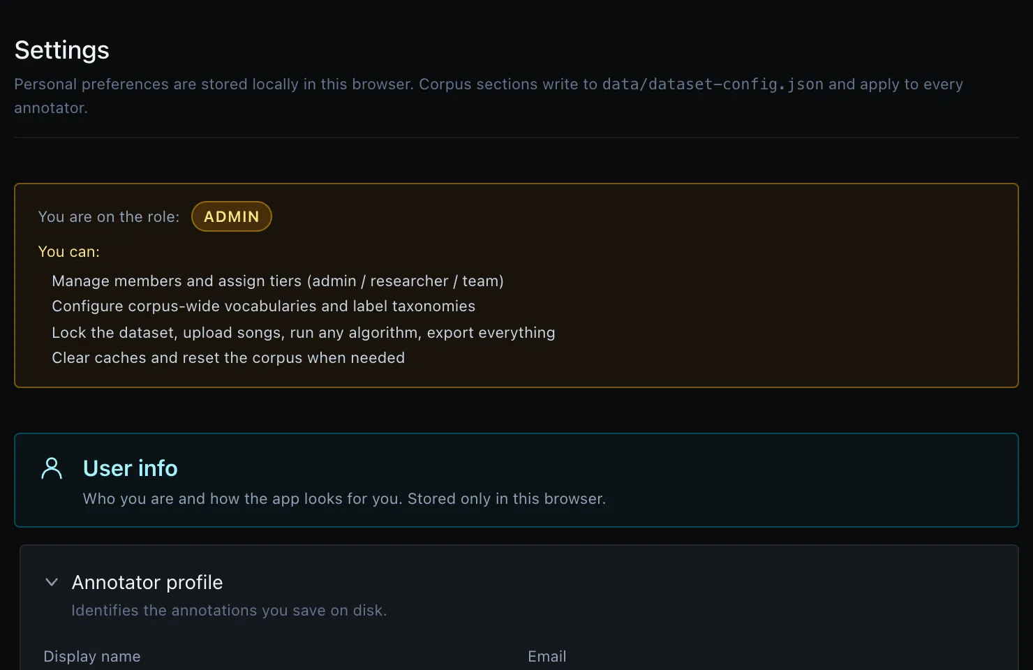The Settings page — the role banner plus the five collapsible, color-coded categories.

Every personal preference and corpus-wide knob is on the Settings page. The page is self-saving — there’s no Save button; a transient Saved pill flashes after every write. Personal preferences land in your browser’s localStorage under timecues.settings.v1; corpus-wide settings (vocabularies, BPM defaults, access list) write through to data/dataset-config.json on the server.

The role banner

A colored banner at the top of the page tells you your current access tier and bullets out what you can do at that tier. Out-of-tier sections elsewhere on the page stay visible (so you know what’s there) but are interaction-suppressed with an Admin only pill.

Tier	Banner accent	Headline capabilities
Admin	amber	Manage members, configure corpus-wide vocabularies, upload/export, clear caches, factory-reset the corpus.
Researcher	violet	Full corpus access, run any algorithm, view every annotator’s output, upload/export. Cannot manage members or change dataset defaults.
Team	cyan	Full corpus access for your own annotations. Cannot see other annotators’ work or run admin actions.
Public	slate	Annotate the shipped default songs only. Other corpus features unlock once an admin adds you to the team.

The five categories

Below the banner the page is grouped into five color-coded collapsible categories. Only Annotator profile is expanded by default — click any other section’s chevron-and-title to open it.

👤 User info (cyan)

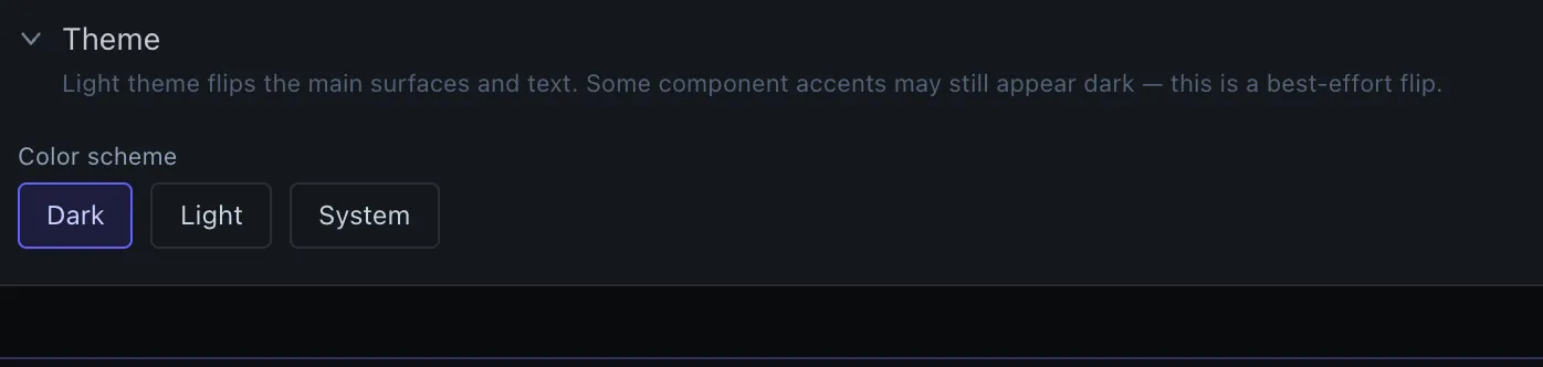User info — your Annotator profile plus the dark / light / system theme switch.

Panel	Tier	What’s inside
Annotator profile	all	Display name, email (auto-filled from Google sign-in), free-text role and affiliation, read-only id + auth method. Requires clicking Save profile (the only setting on the page that’s not auto-saving).
Theme	all	Color scheme radio — dark / light / system. Default dark. system follows your OS prefers-color-scheme.

✎ Annotation (indigo)

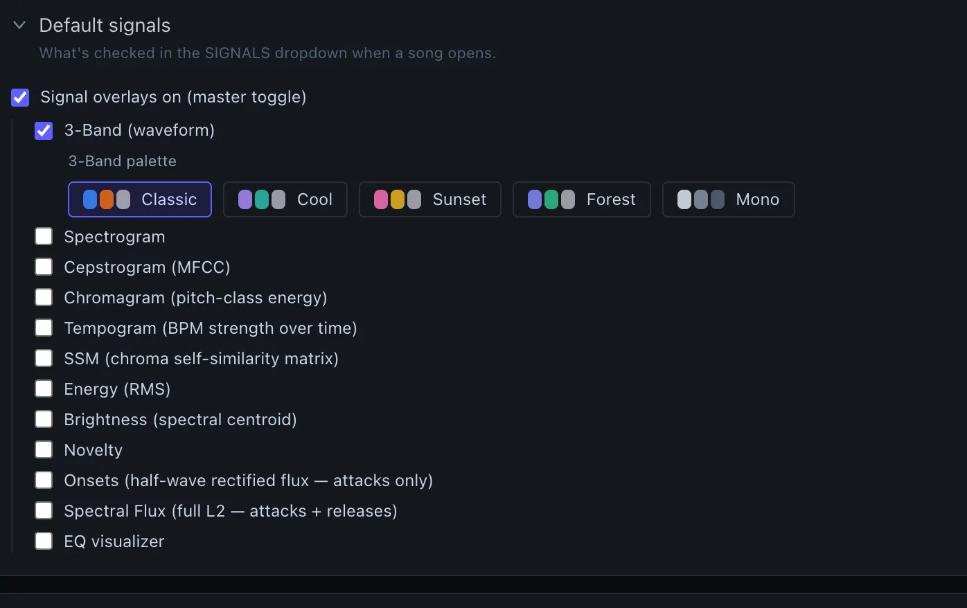Annotation — the master overlay toggle, the twelve signal-row defaults, and the 3-Band palette.

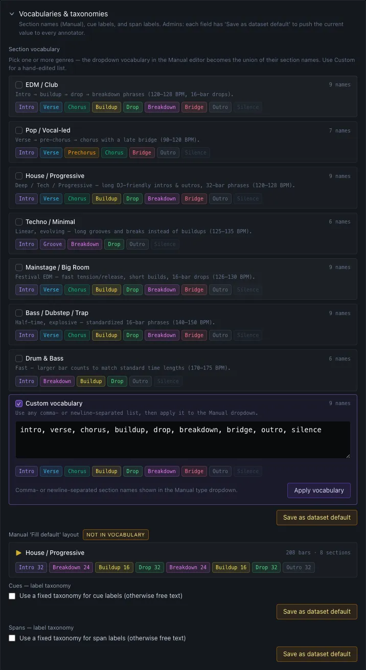Vocabularies & taxonomies — section, cue, and span labels, each with inline (admin) dataset-default controls.

Everything that customizes how you personally see the workspace and the annotation editors. Strictly browser-local — nothing here syncs to the corpus.

Panel	What’s inside
Display & playback	Sidebar collapsed by default, show beat grid by default, default playback rate slider (0.5× – 2.0×, step 0.05, default 1.00×).
Default signals	Master “Signal overlays on” toggle plus 12 sub-toggles for which signal rows are pre-checked in the SIGNALS dropdown (3-Band waveform, Spectrogram, Cepstrogram/MFCC, Chromagram, Tempogram, SSM, Energy/RMS, Brightness, Novelty, Onsets, Spectral Flux, EQ). Plus a 3-Band palette picker (Classic / Cool / Sunset / Forest / Mono).
Annotations — display	Per-layer visibility defaults (Manual / Auto-guess) plus a time-unit picker for annotation editors (Milliseconds or Beats & bars).
Vocabularies & taxonomies	All label vocabularies in one place. Section vocabulary (genre cards plus a custom textarea), cue vocabulary, span vocabulary. Each row has a Save as dataset default / Clear dataset default button visible only to admins, plus a Local override pill that appears next to your row when your local value diverges from the admin default.
Loops	Default loop names, default cue labels for loops, opt-in for the loops marker family (experimental).
BPM & grid protection (personal)	When on, prevents accidental BPM or Grid Offset edits — the field becomes read-only until you toggle it back off. Useful once a song is fully annotated.
Experimental annotation types	Per-family feature flags — Loops, Riff Patterns, Cue Extras, Span layers, etc. Off by default. Switching one on reveals its UI surface across the app.

🔬 Research (violet)

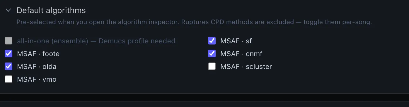Research — which detectors are pre-ticked in Algorithm Inspect, plus BPM-detection and Auto-guess defaults.

Algorithm and detector defaults. Visible to all tiers but read-only for Team / Public — each row carries an Admin only pill at those tiers.

Panel	What’s inside
Default algorithms	Which algorithms are pre-ticked in Algorithm Inspect when a song opens. The order matters — the first ticked algorithm becomes the default reference in the diff readout.
BPM detection	Per-detector enable toggles (client-wabd, librosa-beat-track, librosa-tempo-static, librosa-tempo-dynamic, madmom-rnn-beats, madmom-tempo). Disabled detectors don’t appear in the chip row. Useful for turning off detectors you don’t trust on your corpus.
Auto-guess defaults	Default cluster tolerance τ in seconds (default 3), default minimum agreement count (default 1), default source-detector subset (which of the 30+ detectors feed into Auto-guess by default).
Optional GPU tooling	When the GPU profile is enabled at compose time, toggles here let you opt specific algorithms (allin1, demucs) into GPU acceleration. No effect when the profile is off.

🛡 Corpus management (amber)

Admin & access — the corpus display name and the per-email four-tier People list.

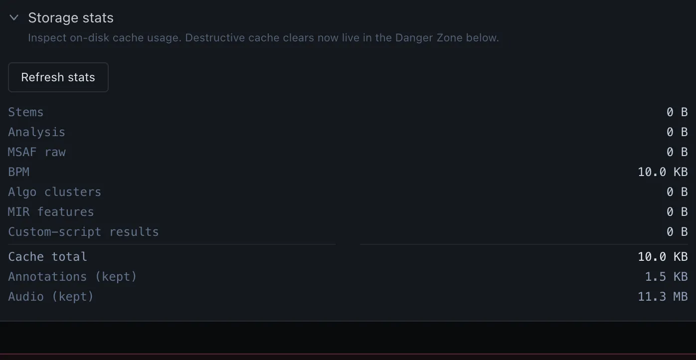Storage stats — on-disk usage by data bucket, plus export and per-category cache clears.

Admin-only. Every panel here writes through to the server (i.e. to data/dataset-config.json) and affects every annotator.

Panel	What’s inside
Admin & access	The corpus’s display name, plus the People list — one row per email, four-tier dropdown (admin / researcher / team / public). Adding an email here is what unlocks an annotator on first sign-in. Removing an email demotes that annotator to Public the next time they sign in.
Storage stats	A read-out of total disk usage by data/ subtree (songs, annotations, algorithm-outputs, stems, song-info), plus an Export everything button (JSON / Audacity / Sonic Visualiser / JAMS / MIDI / REAPER) and per-category Clear cache buttons.

Corpus-wide vocabulary defaults used to live here in a standalone Dataset defaults — corpus-wide vocabularies section. That was retired in 2026-05-18 — every admin “Save as dataset default” / “Clear dataset default” button now lives inline under the field it applies to in Annotation → Vocabularies & taxonomies.

⚠ Danger Zone (rose)

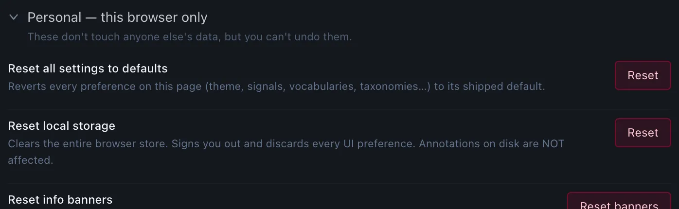Danger Zone — Reset to defaults, a personal reset that only affects this browser.

Danger Zone — corpus-wide destructive actions (clear caches, factory-reset), admin only.

Destructive actions, split in two:

Subpanel	Who can use it	What’s there
Personal — this browser only	all	Reset to defaults — wipes timecues.settings.v1 and restores every preference to the values in DEFAULT_SETTINGS. Annotator profile is unaffected (it’s stored elsewhere).
Corpus-wide — affects every annotator	admin only	Clear all algorithm caches, Clear all annotations for one annotator, Factory-reset the corpus (drops the People list, vocabularies, defaults — leaves audio and annotations intact).

Self-save and the “Saved” pill

Every change other than Annotator profile commits immediately. The Saved pill flashes for ~600 ms top-right after a write so you know the value persisted. There’s no “discard changes” — undo is by re-toggling, or by Reset to defaults in the Danger Zone for a wider revert.

Where settings actually live

Scope	Storage
Personal preferences	localStorage key timecues.settings.v1 (one JSON blob).
Annotator profile	AnnotatorContext — separate localStorage key, requires Save profile click.
Dataset defaults + People list	data/dataset-config.json on the server. Edits via the inline admin buttons hit PUT /api/dataset-config.
Authentication	Google OAuth session cookie. Cleared on sign-out.

Common tasks — where to click

• Make spectrogram on by default → ✎ Annotation → Default signals → toggle Spectrogram on.
• Switch the workspace to light mode → 👤 User info → Theme → radio: light.
• Add a researcher to the team → 🛡 Corpus management → Admin & access → Add row, type email, tier dropdown → researcher.
• Lock BPM on a finalized song → ✎ Annotation → BPM & grid protection (personal) → toggle on.
• Make madmom-rnn-beats the only BPM detector → 🔬 Research → BPM detection → toggle every other detector off.
• Add a custom section label like pre-chorus to the corpus → ✎ Annotation → Vocabularies & taxonomies → Section vocabulary → Custom card → edit the textarea → (admin) Save as dataset default.
• Export the whole dataset to JAMS → 🛡 Corpus management → Storage stats → Export everything → JAMS.
• Reset my preferences but keep my annotations → ⚠ Danger Zone → Personal — this browser only → Reset to defaults.

Deep dive: Settings — the full reference in the user guide enumerates every key, default, and the underlying storage shape.